Decline for Unconventional Reservoirs

Introduction

A limited discussion on applications of various types of decline approaches for shale and/or tight gas.

Modified-Hyperbolic Relation

With the development of unconventional shale reservoirs, choosing only hyperbolic decline could cause an overestimation of estimated ultimate recovery. This is because hyperbolic decline without limit tends to overestimate cumulative production during the life of a well. As a result attempt to account for this, a modified hyperbolic decline can be used in unconventional shale reservoirs and reserve booking.

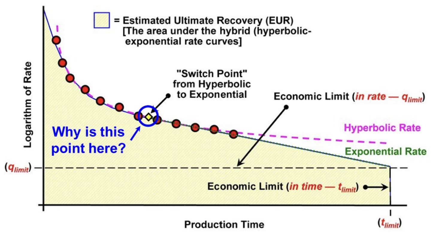
Worked presented by Ilk [2014,2023] suggested that the “Modified-Hyperbolic Relation“ was one of the most common methods to estimate ultimate recoveries (EUR) in unconventional reservoirs. In the image below, this method has a transition from Hyperbolic to Exponential. According to Ilk, each decline curve model can be described as empirical (with no direct link with theory) and generally center on a particular flow regime and/or characteristic behavoir. In general, DCA is not fully representative.

Of course, like other Arp’s or other methods, it can still suffer the problem of a non-unique solution yielding a wide variety of results [Ilk, 2023]. Interestingly, Fulford [2016] claimed that Modified Hyperbolic was not a suitable approach for forecasting in unconventional's.

Fulford [2016] /SPEE Monograph 4 “the most likely failed constraint is constant fluid compressibility… this breaks the theoretical link between exponential decline and all gas wells and all oil wells that will ever produced the bubble point“. There is no theoretical justification or convincing empirical validation of the Modified Hyperbolic Model.
“It does not honor the physics of flow during the transient period”

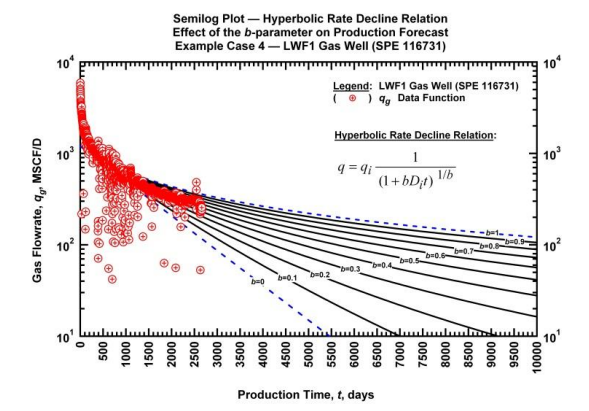
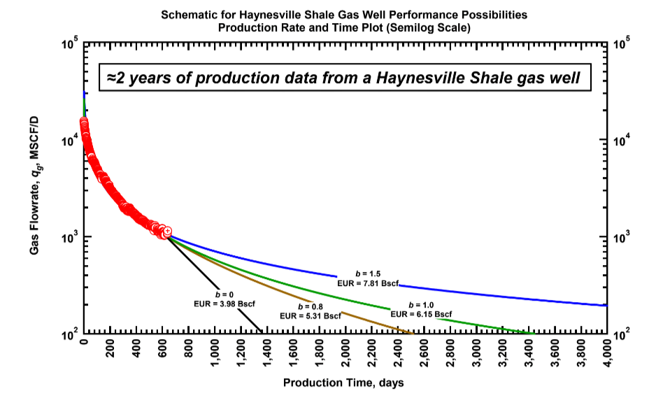
In the example below, three (3) of the four (4) declines are quite suitable, with the fourth (b=0) looking pessimistic - hence, significant uncertainty based on choice of b-value.

Various time-rate diagnostics, as well as Hyperbolic (Arps) and Flow Regime Identification should be used to identify best data for use. According to Blasingame [2017], this approach is highly non-unique in the hands of most users, and often yields widely varying estimates of reserves with time.

According to the literature,, choosing only hyperbolic decline could cause an overestimation EUR. This is because hyperbolic decline without limit tends to overestimate cumulative production during the life of a well. In an attempt to account for this, the modified hyperbolic decline is typically used in unconventional shale reservoirs and reserve booking. Reserve engineers will typically transition a decline curve to an exponential decline to compensate for this overestimation. The transition to an exponential decline in later stages of production is called the terminal decline.

See an interesting field study at Concerns for Type Wells: Infill Drilling, Completion & More and related discussion on child-parent well development.

Modified-Hyperbolic Relation

Blasingame showed the Arps Modified-Hyperboic Decline relations as:

While the following is used for the Exponential Relation:

Where:

t_Lim = the time of the condition is switched.

D_LIM= specified by the analyst

and the following computed according to fit

As the Arps relationship is often used to represent early-time flow behavoir (which will overstimate EUR), the adoption of a protocol to constrain the ultimate extrapolation by splicing a terminal decline trend to a hyperbolic one.

Stretched Exponential Decline Model (SEDM)

The stretched exponential decline method is a variation of the traditional Arps method, but is better suited for unconventional reservoirs due to its bounded nature. That is, for positive inputs, the model gives a finite value of EUR even if no abandonment constraints are used in time or rate (this is very similar to Probability Density Function methods). According to Blasingame [2017], the stretched exponential model is recommended approach for tight gas and shales.

The basic math:

Where:

Tau = Characteristic time parameter

n = Exponent parameter is SEPD model, similar to “b” factor in Arps model, dimensionless

According to Kanfar and Wattenbarger [2012], the first term inside the brackets is the complete gamma function, while the second term is the incomplete gamma function.

For an individual well, the SEDM model parameters, can be determined by the method of least squares in various ways, but the inherent nonlinear character of the least squares problem cannot be bypassed. To assure a unique solution to the parameter estimation problem.

However, as noted by Valko and Lee, decline ratios provide a stable method to solve SEDM parameters (as opposed to Error Minimization). Using cumulative ratios provides a more transparent method to solve for SEPD model parameters and helps prevent a few anomalous points from having undue influence. Specifically, one can solve two equations for two unknowns. Thereafter, one could solve for qo

For practical purposes, the variable n ranges from 0.1 to 1.0, and an n value of 1.0 corresponds to a exponential decline (n = 0. 1 is a very flat decline. The figure below shows a visual interpretation of the parameter n while Tau is held constant.

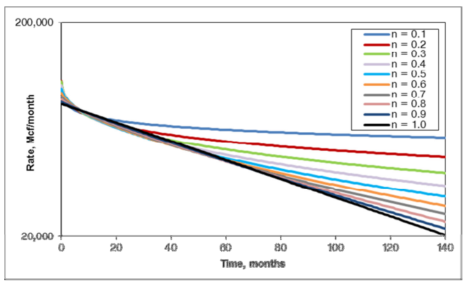
The practical range for the parameter τ has not been well established. While Valko and Lee never used values greater than 1.0 in their work with Barnett Shale wells, there was o evidence to suggest it should be constrained to 1.0 according to Statton ( 2012). Statton did extensive simulation work to help establish proper limits although not discussed here.

According to the literature, the SEDM is the basis for the power law model.

Power-Law Exponential Model

The basics of the power law formulation is shown below. According Blasingame [2017] , it is the most suited tight gas/liquid-rich shale reservoirs. Conceptually, the power-law exponential decline assumes that the b factor trend (I.e. the derivative of the loss ratio) declines as a function of time.

Where:

Although the algebra is not shown here, the solution below shows that the traditional Arps “b“ parameter becomes essentially time dependent [Blasingame 2011]

The image below (the loss Ratio) shows a power law trend observed from shale gas data, and illustrates the power law trend.

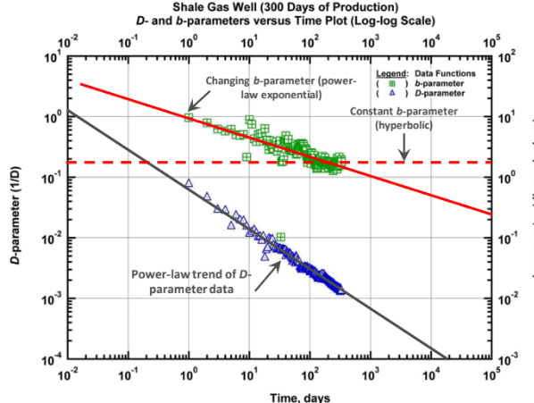
In the work below, credited to Ilk [2017], continuously changing EUR as a function of time due to declining b-exponent. Declining EUR with time is characteristic of the declining b(t) function wtih time.

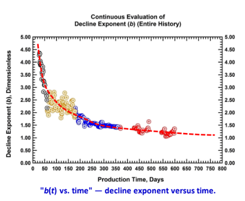
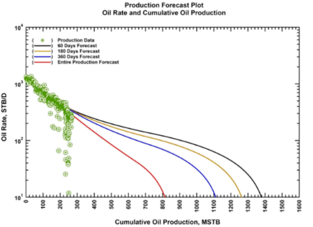
Fun Facts?

Blasingame [2015]

Power-Law Exponetial (PLE) and Stretched Exponential (SEM) are the same when D_infi =0.
The PLE modl was dervied from field Observations (Blasingame/IIk)
The Stretched Exponential was based on statistical texts (Valko)

Comparison of Decline Models to Ideal Model

Erdle [2017] published his findings on comparison of the various decline models to the ideal model.

Model	Low Permeability	Transient Flow	BDF	Change Parameters with Time	Use with < 1 yr data	Easy for Economics
Arps	No	No	Yes	Yes	No	Yes
Arps - Modified Hyperbolic	Maybe	Maybe	Yes	Yes	No	Yes
Streteched Exponential	Maybe	Maybe	No	Yes	No	No
Extended Power Law	Maybe	Maybe	yes	No	No	No
Linear Flow	Maybe	Maybe	No	Yes	maybe	No
Duong	Maybe	Yes	No	Yes	maybe	No
Duong	Maybe	Yes	Yes	No	maybe	No

Derivative Methods & Plots

Ilk [2023] also discussed the Beta-Derivate as a method for identifying power-law flow-regimes in unconventional reservoirs.

Re-arranging for the loss-ratio

Finding the derivative of the loss-ratio

According to Okuma et al [2012], the Beta Function relates rate and the derivative functions as shown in the

two example plots are shown below:

As demonstrated in the plot below, continuous evaluation of b-factor as measured data increases with time. b-values start out high and slowly decrease towards 1 and 0.9

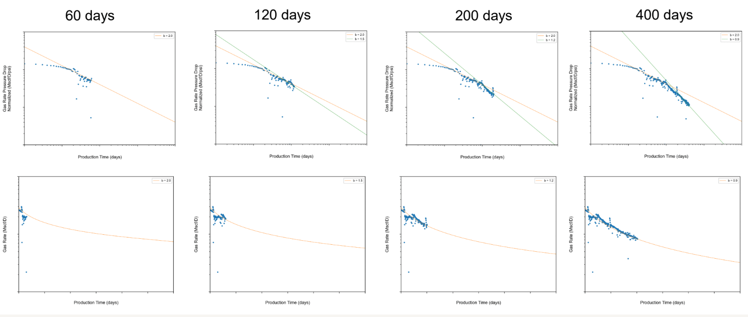
“Pseudo” RTA Methods“

This include methods of:

Basic Pressure Normalized Decline Analysis
The Rate Integral Function which effectively 1/3 of Blasingame Curve without the pressure or time transformations.

References:

Hoss Belyadi, Ebrahim Fathi, Fatemeh Belyadi, Chapter Seventeen - Decline Curve Analysis, Hydraulic Fracturing in Unconventional Reservoirs, Gulf Professional Publishing, 2017,
Dr. Dilhan Ilk, A , Survey on Diagnostic Based Methods for Well Performance Analysis and Production Forecasting in Unconventional Reservoir, SPEE Denver Chapter, April 12, 2023
Petroleum Engineering 613 - Natural Gas Engineering: Lecture 8 Decline Curve Analysis for Gas Wells. T. A. Blasingame, 2021.
Practical Considerations for Decline Curve Analysis in Unconventional Reservoirs — Application of Recently Developed Time-Rate Relations, V. Okouma, N. Hosseinpour-Zonoozi, D. Ilk,, T.A. Blasingame, SPE 162910.
Application of the Stretched Exponential Production Decline Model to Forecast Production in Shale Gas Reservoir, Texas A&M Thesis, Master of Science.
Valko, P.P. and Lee, W.J. 2010. A Better Way to Forecast Production from Unconventional Gas Wells. Paper presented at the SPE Annual Technical Conference and Exhibition, Florence, Italy. Society of Petroleum Engineers 134231-MS.
Engineering Aspects of Unconventional Oil and Gas Reservoirs, T. A. Blasingame, 11 May 2011, Crisman Institute Shale Gas Meeting
Modern Time-Rate Relations, Lecture 17, Petroleum Engineering 648 - Pressure Transient Testing. T. A. Blasingame.
T.A. Blasingame, Pressure Transient Analysis (PTA) , Rate Transient Analysis (RTA) & Decline Curve Analysis (DCA) Methods for Wells in Unconventional Reservoirs. SPE Denver Section. General Meeting 16 December 2020
Jim Erdle, “An Overview of SPEE Monograph # 4 “Estimating Ultimate Recovery of Developed Wells in Low-Permeability Reservoirs”, 16 May 2017, Ryder Scott Conference.
David Fulford, Machine Learning for Production Forecasts: Accuracy Through Uncertainty. 12th Annual Ryder Scott Conference. Sept 14, 2016.
Engineering Aspects of Unconventional Oil and Gas Reservoirs, T. A. Blasingame, 08 July 2015, SPEE Lunch Presentation.
M. Kanfar & R.A. Wattenbarger, Comparison of Empirical Decline Curve Methods for Shale Wells. SPE Canadian Unconventional Resources Conference held in Calgary, Alberta, Canada, 30 October–1 November 2012.