
Introduction
This module will also a user to perform Monte-Carlo simulation for both multiple measures, and multiple seams.
AFA requires at least 1 Project and 1 Group to perform any analyses or simulation. Please refer to Create a Project and sub-topics if required.
NOTE: AFA use’s Weighted Percentiles Approach for P10, P50, P90, and Pmean .
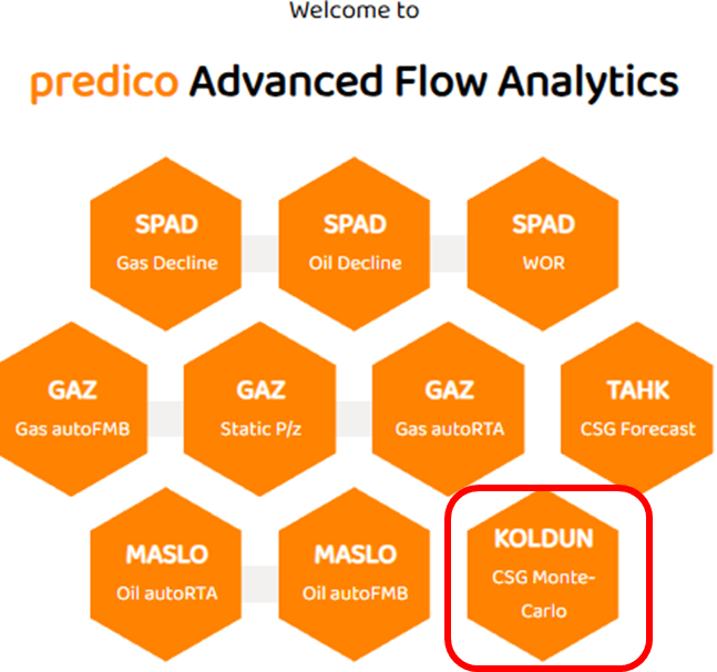
STEP 1: Select the KOLDUN CSG Multi-Carlo Simulation Module
The MC CSG module is to the far right of the AFA Grid.
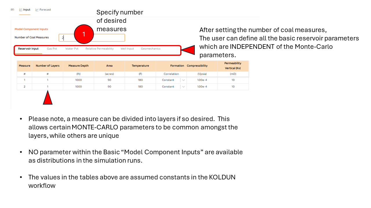
STEP 2: Complete the “Model Components“ Table
In this step, you must specify the number of coal measures and/or layers relevant to your project.
A measure can have 1 or more layers.
If more than 1 layer is specified. Some Monte-Carlo parameters/distributions can be specified for each specific layer while others specified for the measure (if specified for the measure, the Monte-Carlo parameters/distributions are common across multiple layers)
The default PVT Correlations and Calculations are generally suitable for CSG, All values in this table are assumed constant in any simulation run.
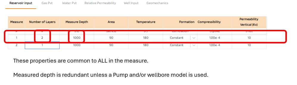
2-1: “Reservoir Input“ Table
-
Specify the number of layers in each measure.
-
Specify the drainage area (or Area) of each measure.
-
Specify the Measured Depth of each Measure
Note: All layers in the Measure will have the same depth, drainage area, PVT and other properties.
Note: The “Measure Depth” values are irrelevant in some scenarios, such as assuming constant bottomhole pressure or no wellbore model. See also CSG Pump & Wellbore Options
Note: Read Coal Measure vs Coal Layer for clarification of these definitions.
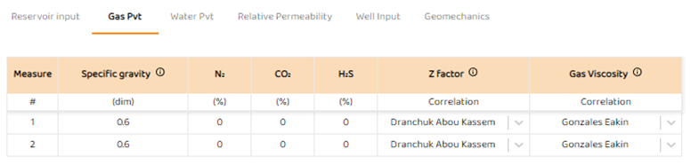
2-2: “Gas PVT“ Table
-
Specify gas gravity and impurities
-
Specify desired gas correlations to use in the calculations.
Note: All layers in the Measure will have the same depth, drainage area, PVT and other properties.
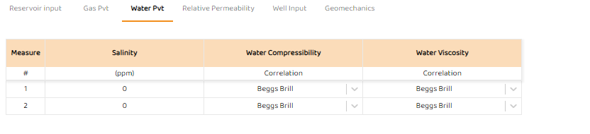
2-3: “Water PVT“ Table
-
Specify Water Salinity
-
Specify desired correlations
Note: All layers in the Measure will have the same depth, drainage area, PVT and other properties.
2-4: “Relative Permeability“ Table
-
Specify Relative Permeability Parameters
Note: All layers in the Measure will have the same depth, drainage area, PVT and other properties.
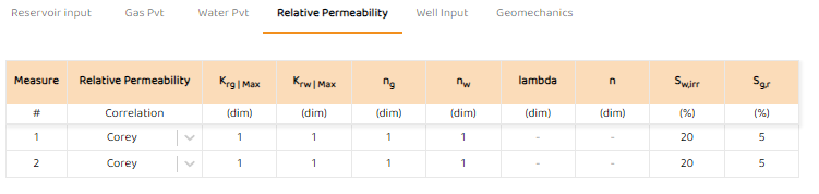
Engineering Tip
-
For “X“ curves, one typically sets ng and nw = 1.0 (using Corey curves)
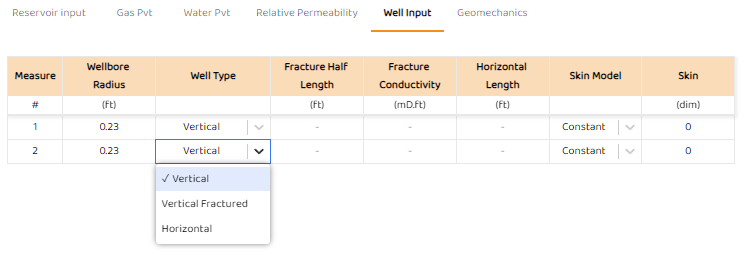
2-5: “Well Input“ Table
The Well Input table is where you select your desired completion which may include:
-
Vertical Wells
-
Finite Conductivity Fractures
All of these models are PSS Models as opposed to Transient Models & Flow Regimes
If inputs in the this table are not applicable to your well completion, they will display “-“ and cannot be edited.
The horizontal well is only available if there is 1 layer in a measure!
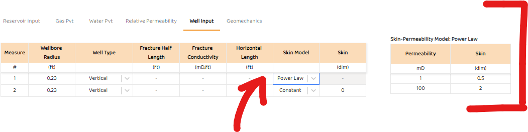
2-5-1: “Skin Model“
Some special consideration to “Skin Model”. The user has two options:
-
Constant skin which reflects Wellbore Skin and Formation Damage per measure
-
This approach assumes each measure (and therefore layer) has a single constant skin
-
Values can be both positive and negative.
-
-
Power Law (see Power Law: Custom Perm - Skin Relationship )
-
This option takes at least two (2) data points {k, skin}
-
The Power Law model assumes a non-linear relationship between permeability and skin.
-
For Monte-Carlo simulations, skin is function of the permeability (skin =f(k)) and changes with each new simulation run.
-
Any measure that uses the Power-Law use the same Power-Law Table shown below:
-
STEP 3: Complete “Monte-Carlo Inputs“ Table
The primary view of the for the Monte-Carlo inputs are shown below. We will discuss the following in order.
-
Number of Simulations
-
Specify Input
-
Measure
-
Specifying distributions per layer or per measure.
3-1. Number of Simulations
This input defines how many runs of a particular simulation you want. If you select 1, you will only see a single curve on your plots (regardless of you distribution settings). With a value of 1, you will have effectively created a deterministic model.
3-2. Specify Input
Similar to TAHK: Coal Seam Gas (PSS) Forecast , the user has the option of working with traditional volumetric inputs, or OGIP inputs.
The isotherm properties in AFA can be specified in two options:
-
Traditional Langmuir and Volumetric Inputs - very common to most commercial simulators
-
-
This option does not require detailed knowledge of Langmuir Volume (VL), Coal Density, Desorption Pressure, or or coal impurities.
-
This option will back-calculate the Langmuir Volume (VL), desorption pressure, and coal density from the degree of Undersaturation (Dewatering) (how far from the isotherm at initial conditions) and the initial gas content (GCi).
-
In the OGIP option, Langmuir Volume (VL) and coal density are back-calculated and displayed.
The images below shows the two various options you can use.
-
All volumetric parameters such Coal Density and Isotherm information are specified in Volumetric Inputs. In-situ or as-received CSG properties are assumed.
-
The table below gives basic insight into the two (2) different types of inputs
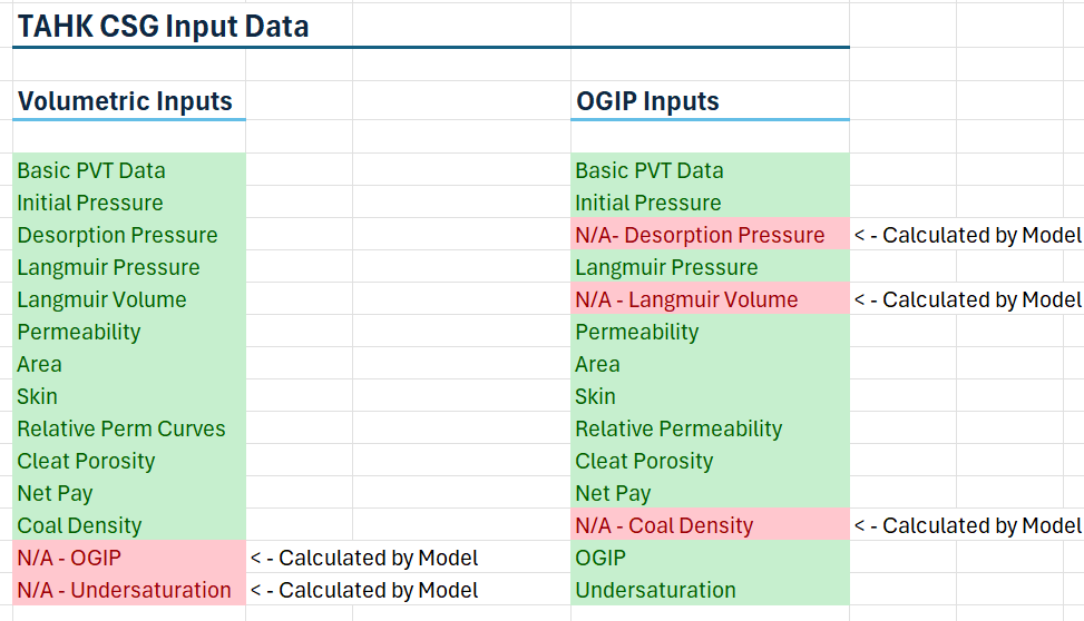
The FINAL selected option, OGIP or Volumetric, will apply to all measures! You cannot mix and max OGIP and Volumetric Inputs during any simulation!
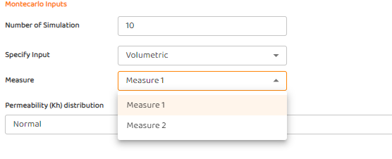
3-3. Measure
When using multiple measures, you can only change distributions for each measure one at a time!
You must select the measure of interest! and adjust the distributions and then move on to the next measure.
The image below shows how the user must select a measure for editing.
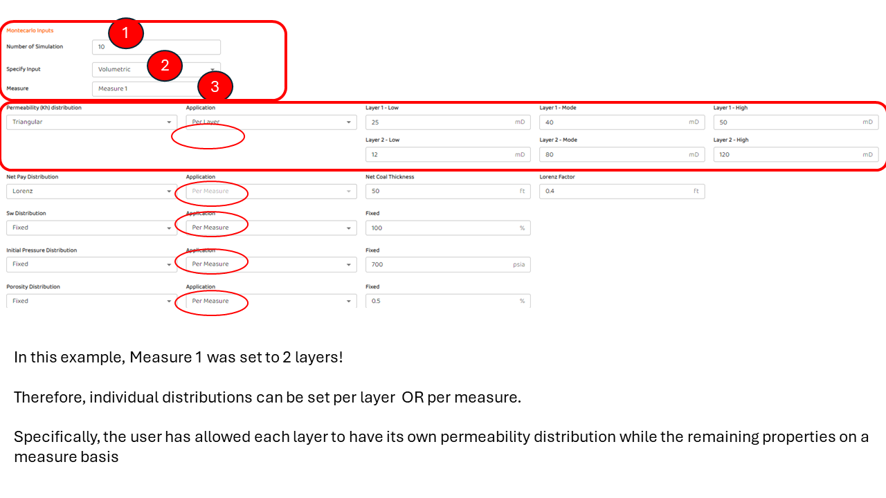
3-4. Using Layer & Measure Distributions
As shown below, the user has selected two layers for Measure 1. Therefore a user can have for a different distribution for each layer - in this case, horizontal permeability is per layer while the other properties are per measure.
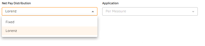
3-5: Select Distribution Type for Each Measure Property
Each property can have a specific distribution. Depending upon the distribution of choice, the various inputs for the selected distribution may change.
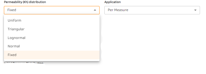
Note: Some distributions only apply to specific parameters. For instance, the The Lorenz Coefficient (Lk) (distribution) is only applicable to “Net Pay”.
With using distributions with high standard deviation, it is possible that conflicting parameters can occur during the monte-carlo.
Refer to Parameter Consistency in Monte-Carlo for how the AFA platform handles such scenarios.
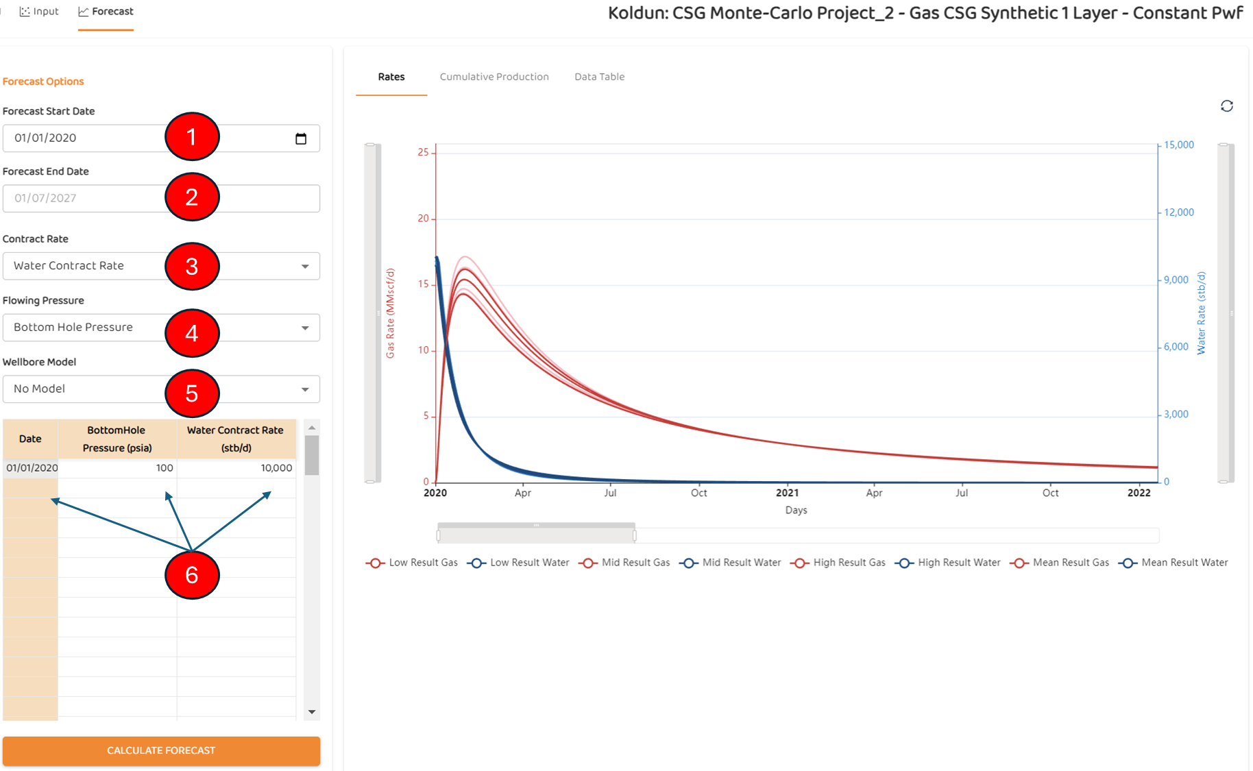
STEP 4: Forecast Tab
The forecast tab, as shown below, has six (6) main components
-
Forecast Start Date
-
Forecast End Date
-
Contract Rate
-
Flowing Pressure
-
Wellbore Model
-
The Forecast Table
Engineering Tips
4-1 Forecast Start Date
This option allows you to STAGE the forecast relative to other wells within the Project as discussed in Create a Project
The project still has its own Start and End Date, but various wells and simulations can start in a sequence if so desired. Refer to the image below:
4-2 Forecast End Date
This is LOCKED and set by the Project settings for all the wells within the project.
4-3 Contract Rate
The user can decide if they wish to constrain production by either gas or water volumes. Simply click and select the desired fluid. In this example, total water production is constrained to 10,000 Bbl/d.
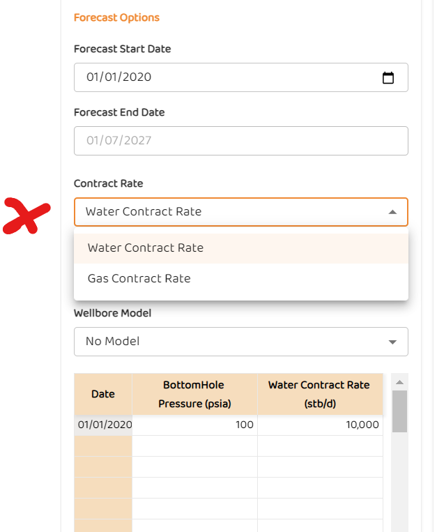
If the total reference fluid does not exceed this value, then it is bypassed (ignored) and the model is flowing pressure constrained.
4-3-1 See also:
Contract Rate (Rate Constraints)
Water Rate Constraint Crossflow Calculations
Gas Rate Constraint Crossflow Calculations
4-4 Flowing Pressure
The flowing pressure is pressure source to be used when generating a forecast.. Refer to the image below:
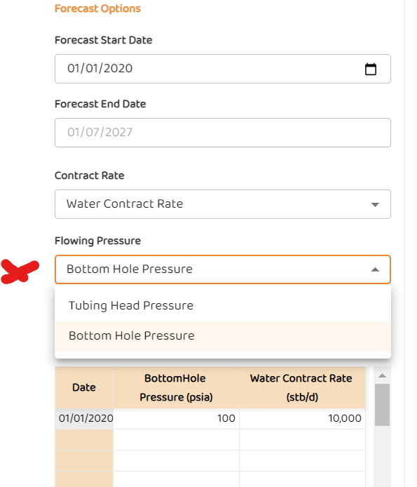
If a user selects a wellhead pressure (casing, tubing, or other), the module will assume these are representative of Bottomhole conditions!
If a user enables a wellbore model, then the wellhead pressure is treated as wellhead pressure in the AFA platform
In the example below, the user has selected “Tubing Head Pressure“ but these values will be assumed to be BHP unless the user selects a wellbore model.
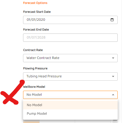
4-5 Wellbore Table
Currently, the user has two options:
-
No wellbore model
-
Pump model which is discussed here at CSG Pump & Wellbore Options.
-
Essentially, the pump model allows fluid movement in the wellbore to be dictated by basic pump specifications.
-
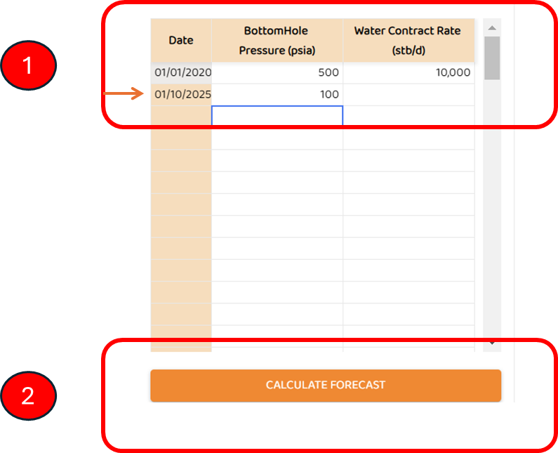
4-6 Forecast Table
The forecast table allows the user to have variable flowing pressures and/or variable production constraints where gas or water volumes.
See Also:
Other Reading:
Weighted Percentiles Approach for P10, P50, P90, and Pmean
Parameter Consistency in Monte-Carlo
CSG Permeability / Permeability Anisotropy