
Introduction
autoRTA is short for automated Rate Transient Analysis.
AFA requires at least 1 Project and 1 Group to perform any analyses or simulation. Please refer to Create a Project and sub-topics if required.
STEP 1: Select the GAZ autoRTA
STEP 2: Data View
Data View is the first tab in most modules. It shows all the major data sources imported for this well (pressures, rates, etc). Some specific items are:
-
Options to select which axis a data set below (left or right)
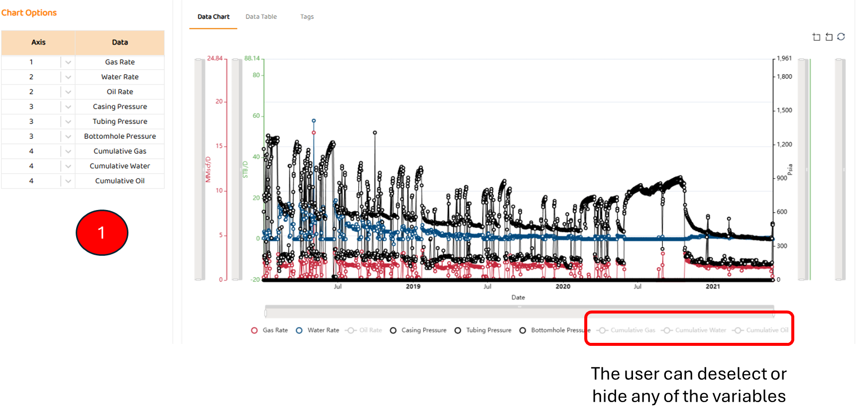
The plots and tables are purely for display, although they can be downloaded as per Downloading Plots and Downloading Tabulated Data .
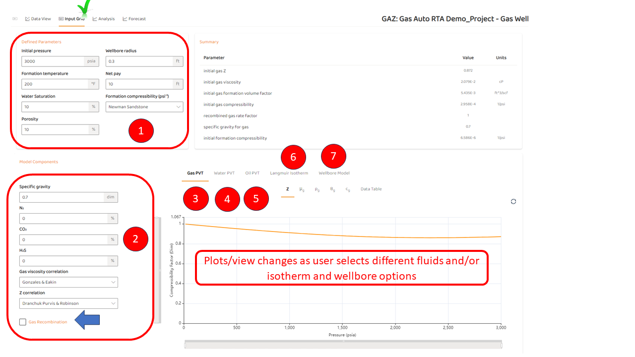
STEP 3: Input Grid
The user must specify all the PVT and rock properties shown below to proceed to the analysis or “Analysis“ tab. On this tab, there are:
-
Defined Parameters
-
These are generally parameters given by the user including
-
-
PVT inputs and general PVT Correlations and Calculations including recombination calculations.
-
Gas PVT Plots - viscosity, density, z-factor etc
-
Water PVT Plots - viscosity, density, etc
-
Oil PVT Plots - viscosity, density, solution GOR, etc (may not be relevant for some gas projects)
STEP 4: Analysis
After all appropriate inputs are completed, and the user clicks the “Analysis“. Key elements are:
-
Outputs from the automated analysis:
-
If “Smart Fit“ is turned off, the user may select any model as they see fit, and perform a manual analysis.
-
-
Normalized Pressure Plots and Tabs
-
Beta derivatives
-
Normalized Rate Plots
-
BlasingamePlots
-
Tabulated “Data Table“ of the results in the dimensionless form
-
Tabulated “Data Table“ of the base model curves
-
Adjustable Dimensionless Time Scale. Options available are:
-
tDrw
-
tDA
-
tDd
-
-
Manual Options such as Dual Porosity and Boundary Type.
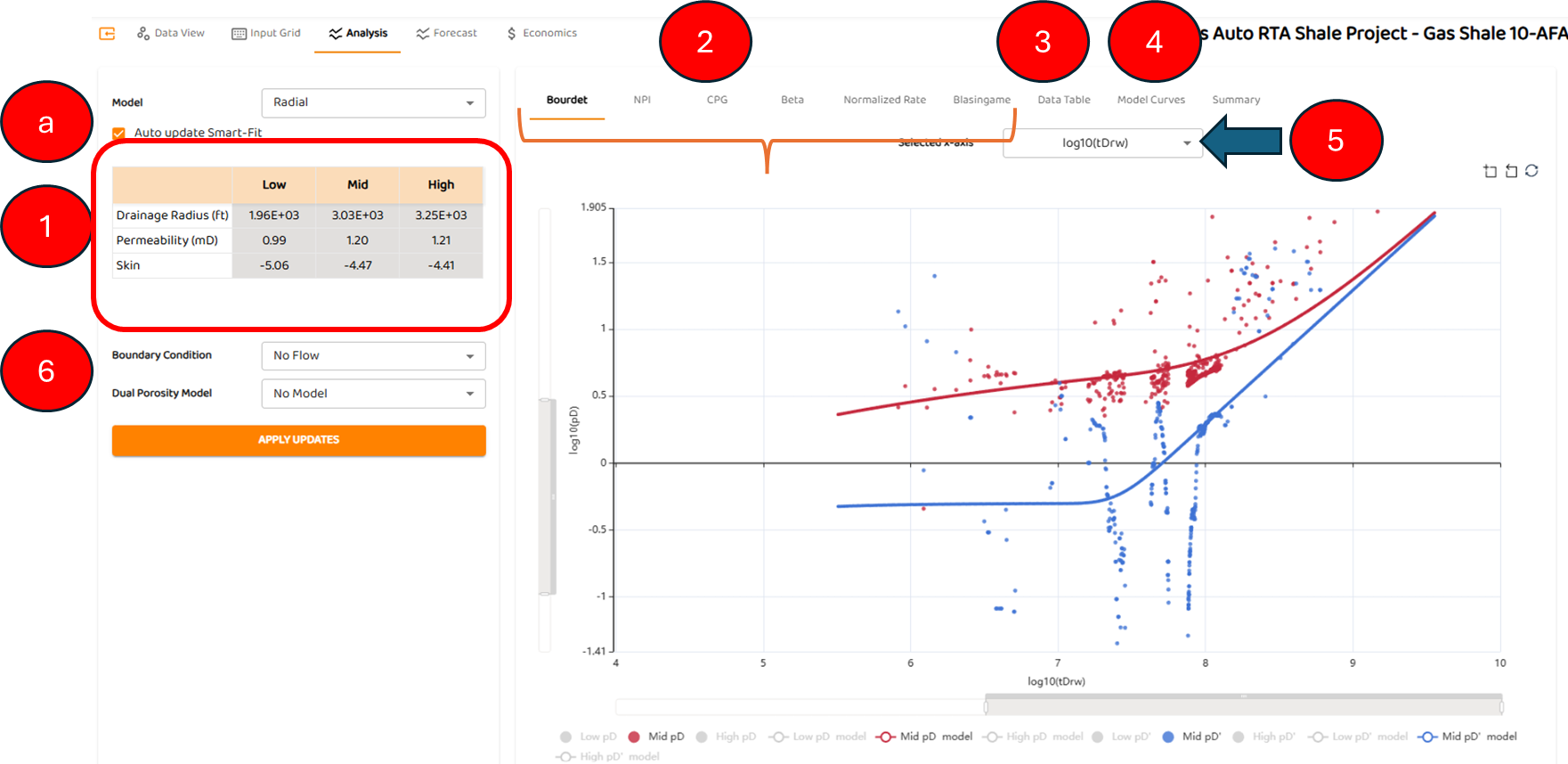
By default, the mid-case analysis for each curve is shown. The high and low cases are turned off until the user selects them from the legends
See here for more about RTA Sensitivities
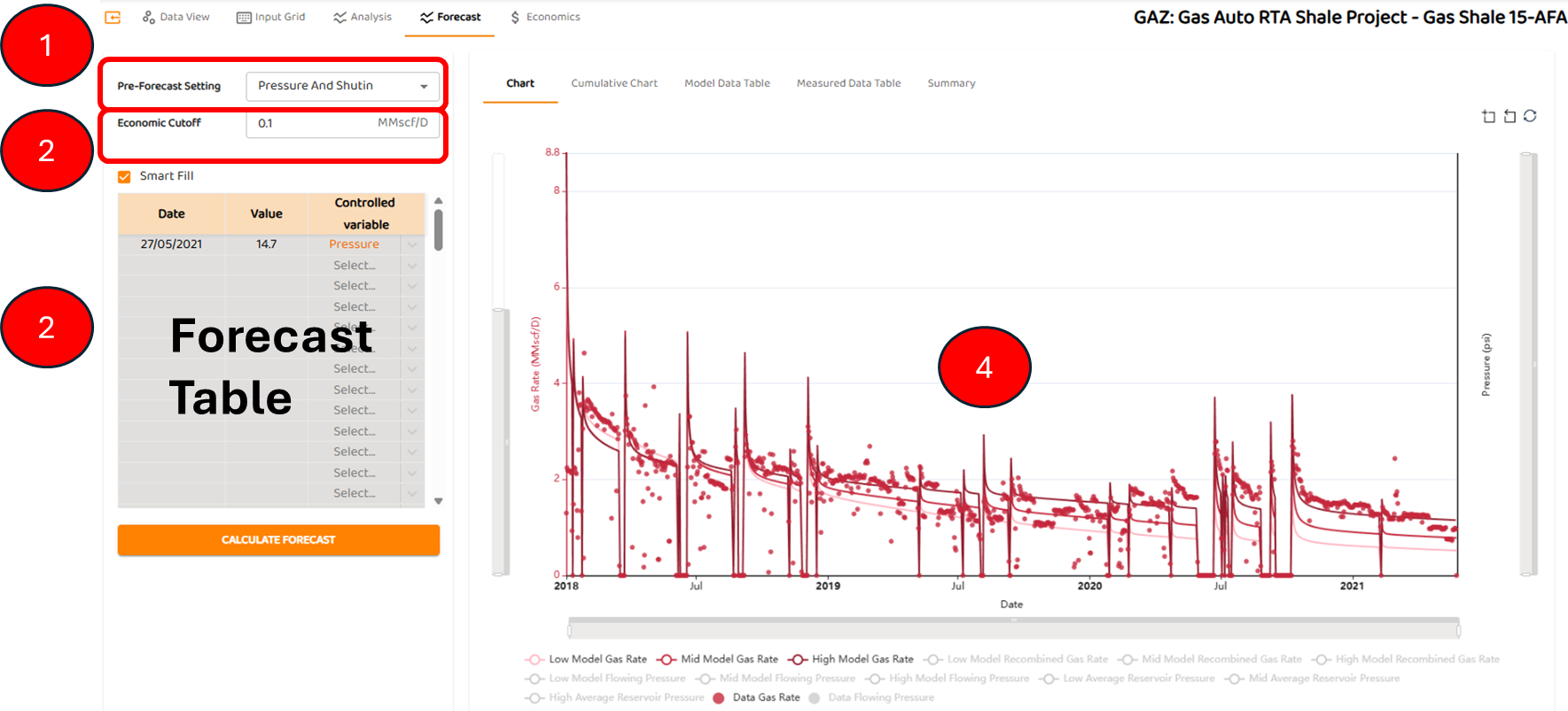
STEP 5: Forecast
When selecting the forecast tab, the results of the analysis and history match are shown. The basic elements are:
-
autoRTA Pre-Forecast Settingwhich gives options for the history match period.
-
Economic Cut-off
-
Forecast Table and Smart Fill which sets the forecast conditions beyond the history match
-
The history match and forecast periods
Also, note all three forecasts (low, mid, and high) from the automated analysis are shown below.
See Also:
See Also: