TAHK: Coal Seam Gas (PSS) Forecast

Introduction

This module will also a user to perform a DETERMINSTIC production forecast for coal seam gas reservoirs with multiple layers. It assumes the use of PSS Models It can be run either as single or multilayer (with crossflow).

AFA requires at least 1 Project and 1 Group to perform any analyses or simulation. Please refer to Create a Project and sub-topics if required.

STEP 1: Select the TAHK CSG Forecast Module

The TAHK Gas Forecast module is to the centre of the AFA Grid.

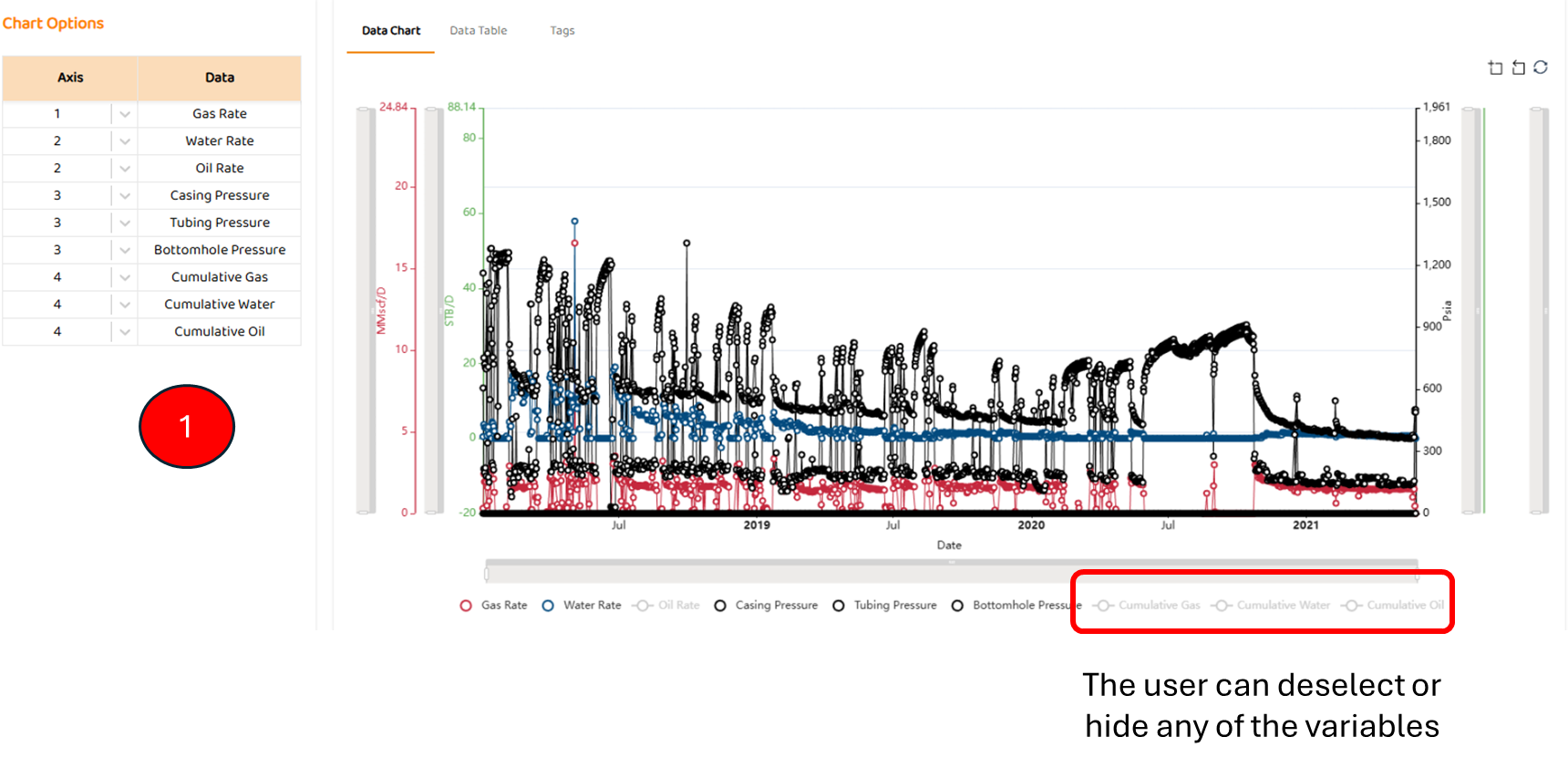
STEP 2: Data View Tab

Data View is the first tab in most modules. It shows all the major data sources imported for this well (pressures, rates, etc). Some specific items are:

1. Options to select which axis a data set below (left or right)

   

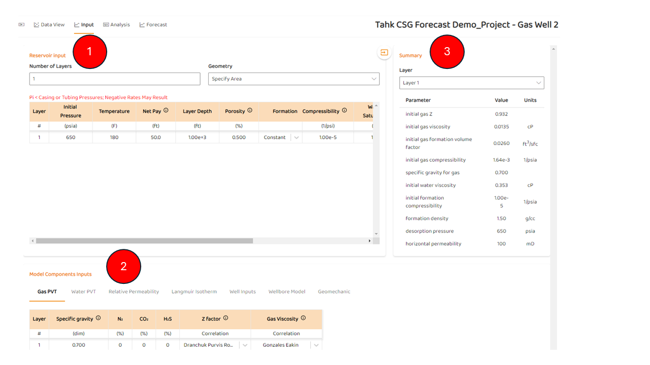
STEP 3: Overview of the Input Tab

After the Data Tab, the user will see the Inputs Tab. The three (3) main components of the Input Tab are:

1. Reservoir Inputs (Per Layer), which include basic petrophysical data:

   1. Number of Layers

   2. initial Pressure,

   3. PVT and compressibility's

   4. net page,

   5. drainage area,

   6. CSG Permeability / Permeability Anisotropy , and more.

2. Model Component Inputs, which include

   1. Isotherm Langmuir parameters.

      1. Please review the additional information further below in STEP 4 as the isotherm can be entered in two very distinct approaches.

   2. Well Completion Type (Well Type). Refer to TAHK Well Options

      1. Vertical Well + skin

      2. Vertical Well + finite conductivity fracture

      3. Horizontal Well Models

      4. Skin options, such as Power Law: Custom Perm - Skin Relationship capability.

      5. Geomechanics models for Stress Dependent Permeability.

      6. Matrix Shrinkage Modelsfor coal.

   3. Wellbore Model with CSG Pump & Wellbore Options

3. Summary Tab

   1. Basic calculated values like z-factor at initial condition

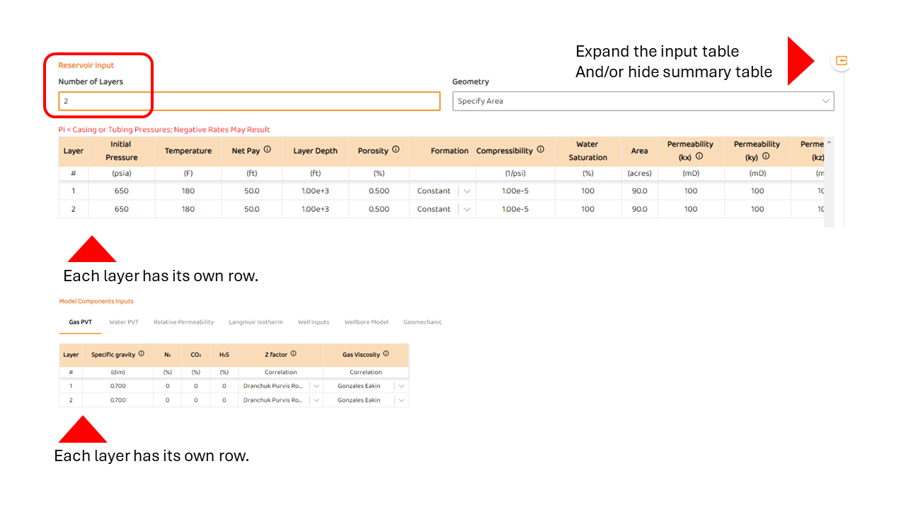
STEP 3: Selecting Single or Multi Layer Option

To use multi-layers, the user simply types a value greater than 1 in the “Number of Layers“ option box as shown below.

All other tables in “Reservoir Input” and “Model Components Update“ by adding additional rows corresponding to each new layer.

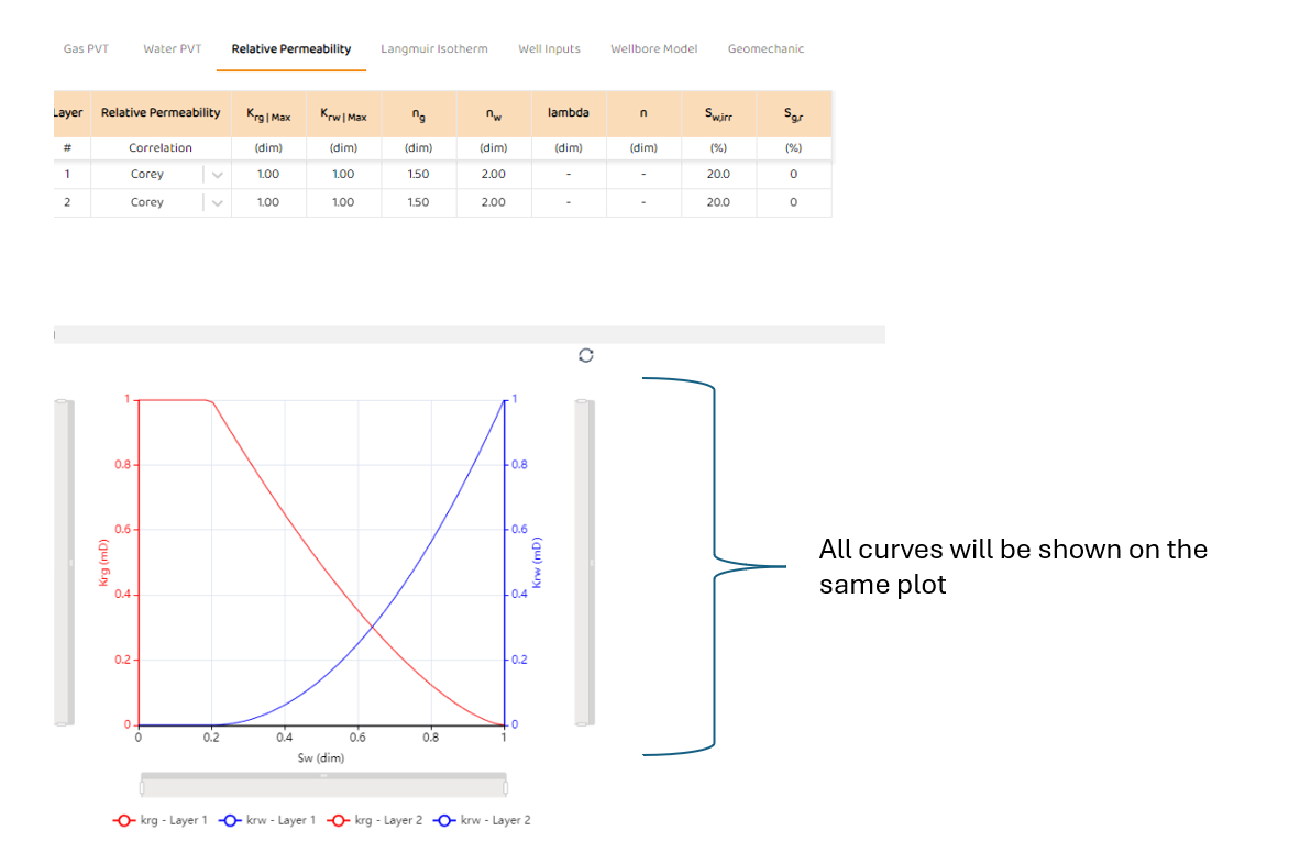
If appropriate, any images or graphs wills show properties for all layers. In the example below, there are two (2) layers and the relative permeability plot shows the model for each layer.

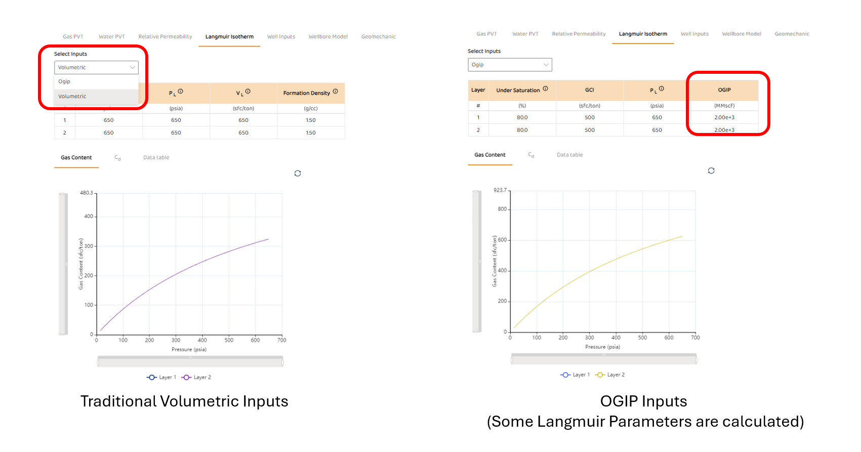
STEP 4: Specifying the “Langmuir Isotherm”

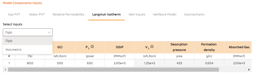
The isotherm properties in AFA can be specified in two options:

1. Traditional Langmuir and Volumetric Inputs - very common to most commercial simulators

2. OGIP Inputs.

   1. This option does not require detailed knowledge of Langmuir Volume (VL), Coal Density, Desorption Pressure, or or coal impurities.

   2. This option will back-calculate the Langmuir Volume (V_L), desorption pressure, and coal density from the degree of Undersaturation (Dewatering) (how far from the isotherm at initial conditions) and the initial gas content (GC_i).

In the OGIP option, Langmuir Volume (V_L) and coal density are back-calculated and displayed.

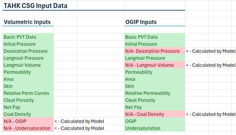
The images below shows the two various options you can use.

1. All volumetric parameters such Coal Density and Isotherm information are specified in Volumetric Inputs. In-situ or as-received CSG properties are assumed.

2. The table below gives basic insight into the two (2) different types of inputs

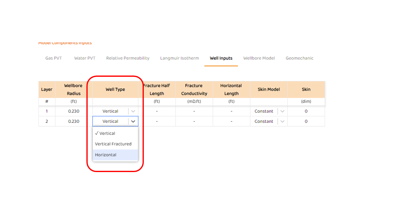
STEP 6: Specify “Well Inputs“

The AFA user can select the type of well completion/geometry in AFA as shown in the image below.

The three (3) current options are:

1. Vertical well + traditional Wellbore Skin and Formation Damage

2. Vertical well + finite conductivity fracture model + traditional Wellbore Skin and Formation Damage

3. Horizontal well

All models used are PSS Models

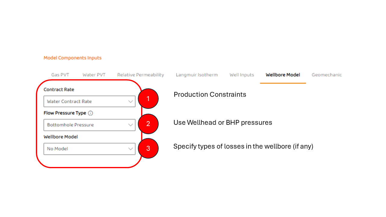
STEP 7: Specify “Wellbore Model“

The AFA wellbore model can has three (3) components.

1. The user of AFA can specify if production can be constrained by either Gas or Water.

   1. The magnitude of constraint will be reflected in the forecast tab, discussed further below.

2. Depending on the data available to any specific well, a variety of pressure types may be available

3. Wellbore model - represents the types of losses in the wellbore. Currently the two options are:

   1. No Model - Assumes any pressure type specified in 2) is representative of all layers

   2. Pump Model - Using basic pump details, the a fluid is drawn down at a user determined rate.

      1. For more details on the pump, go to CSG Pump & Wellbore Options for specific details on how to use this model

         

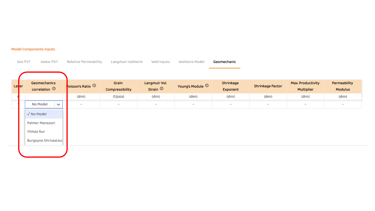
STEP 8: Select “Geomechanic Tab“

In AFA, the user may select different types of models for stress dependent permeability, matrix shrinkage, or even a combination. Currently, there three (3) basic options which include:

1. No model - basic geomechanics is ignored

2. Palmer Mansoori Model - a traditional SDP/matrix shrinkage model often discussed in the literature

3. Yilmaz - Nur model - a basic SDP model

4. Burgoyne-Shrivastava - An Australian model derived and tuned to Eastern Australian data.

   

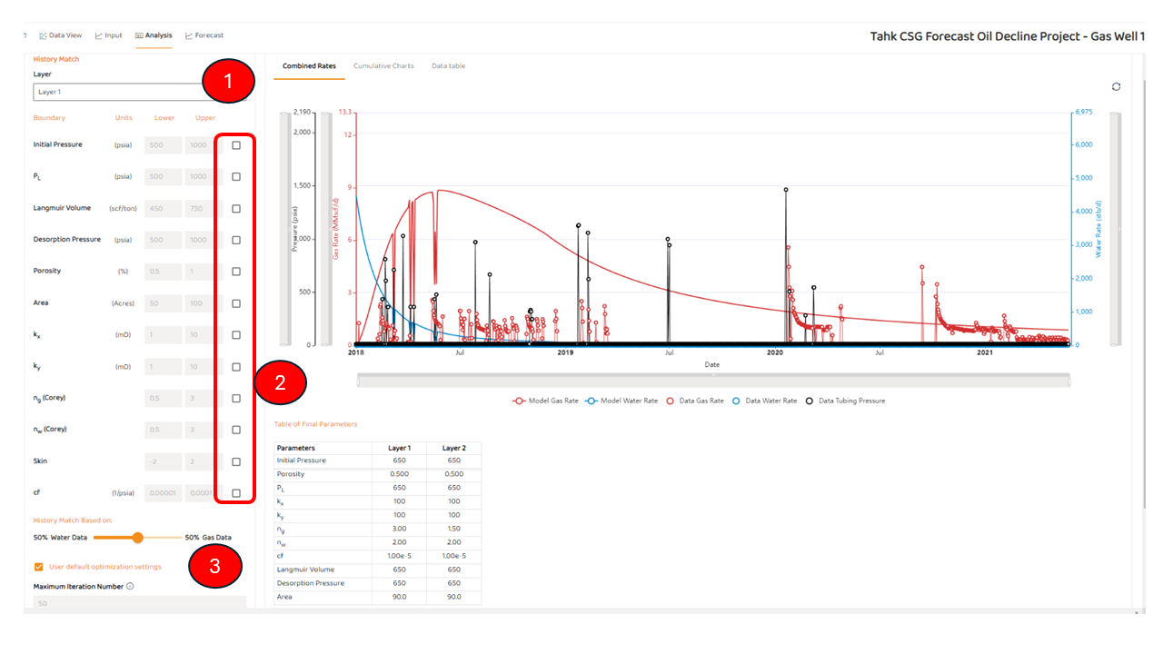
STEP 8: Analysis Tab (& Automated History Matching).

The analysis tab in TAHK CSG actually performs the history match using specified parameters from Inputs Tab (see above). The main components are

1. The layer for which are you selecting parameters for automatic history match. If you have more than 1 layer, the user must select parameters for each layer.

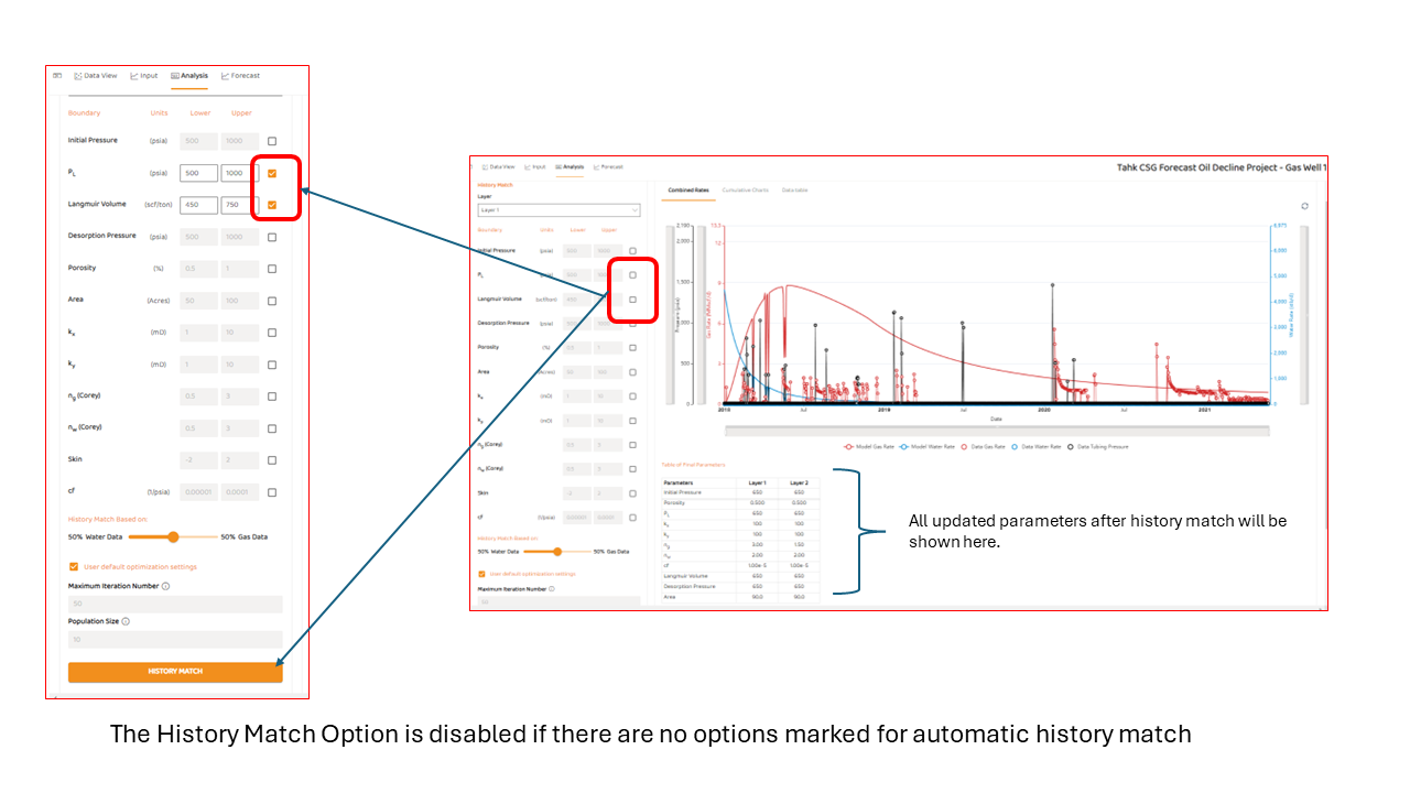
2. Selection boxes, these boxes (and associated ranges) are the values and parameters you wish to history match with.

3. Emphasis on Gas or Water, or a combination in between. AFA has the flexibility to focus on both phases, or individual phases.

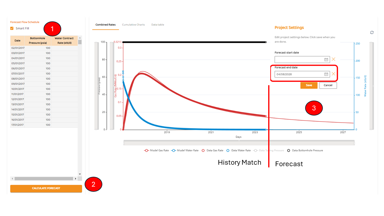
STEP 6: Forecast Tab

Assuming a Set Forecast End Date operation was performed, there are three (3) main parts of the Forecast Tab:

1. “Smart Fill“ - AFA will populate the forecast schedule and use an average of the measured flowing pressures for the forecast.

2. “Calculate Forecast“ - If the user clicks, it will generate the history match, and the following forecast.

3. A forecast will appear which goes the forecast end date.

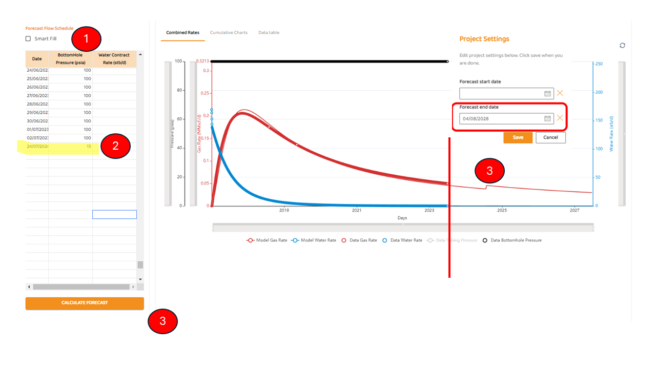
if the user wants to specify future operating conditions such as BHP or a contract rate of some sort, then they must perform the following:

1. They must disable “Smart Fill”

2. They must SCROLL to the bottom of the existing table, and enter the date of the pressure and/or contract rate change as shown in YELLOW in the figure below.

3. Press “Calculate Forecast“

See Also: