
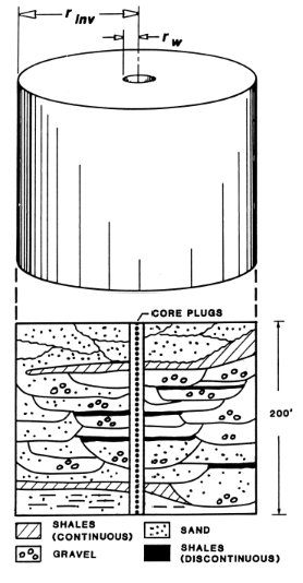
According to Blasingame[n.d.], production data analyses and pressure transient analyses “see“ the reservoir as a volume-averaged set of properties (see image below). In AFA terminology, the terms “Equivalent Radial Homogenous Reservoir” is often used. As new analytical models or solutions are developed, they will have the same view of the reservoir.
Below, the images, taken from Halderson, show conceptual scales associated with porous media mediate averages (left), and pressure-buildup “view“ of relatively large-scale internal heterogenities.
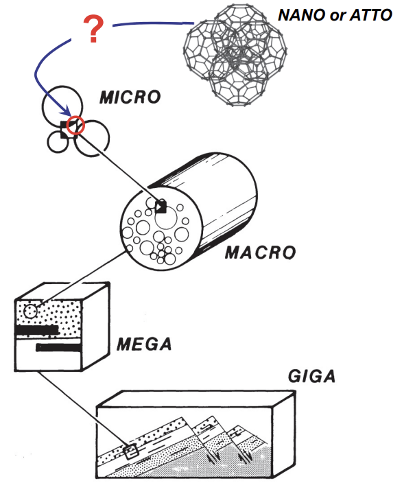
Micro = Scale of pores and grains
Macro = Scale of conventional core plugs
Mega = Large grid blocks in simulation models
Giga = Total formation or regional scale.
This problem is independent of the quality or type of PTA/RTA model; in other words, new solutions will also have this view of the reservoir. When using various transient and/or PSS models, one must understand the scale of the reservoir features. AFA often uses the term “Equivalent Homogeneous Reservoir“ model to describe this phenomena.
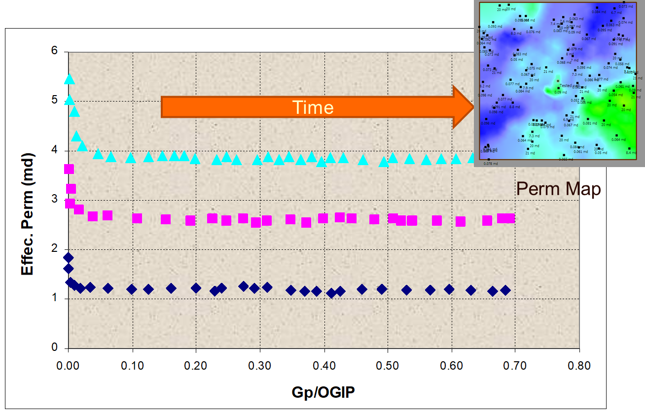
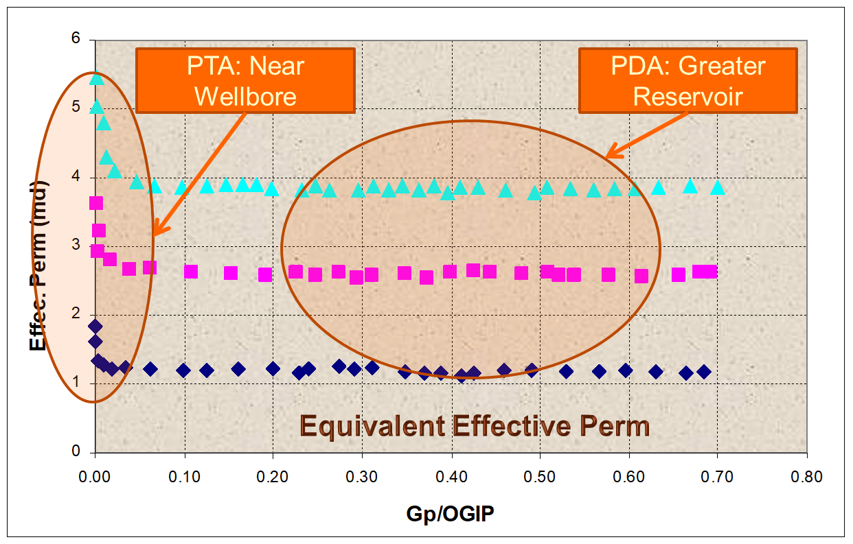
Jordan (2009) performed a number of simulated examples with variable permeability and produced the conceptual plots below, which showed
-
As a general rule, the effective permeability derived from PTA started high, and reduced towards a constant as production (or time) approach PSS.
Internal Boundary Example
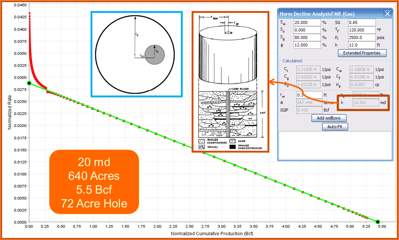
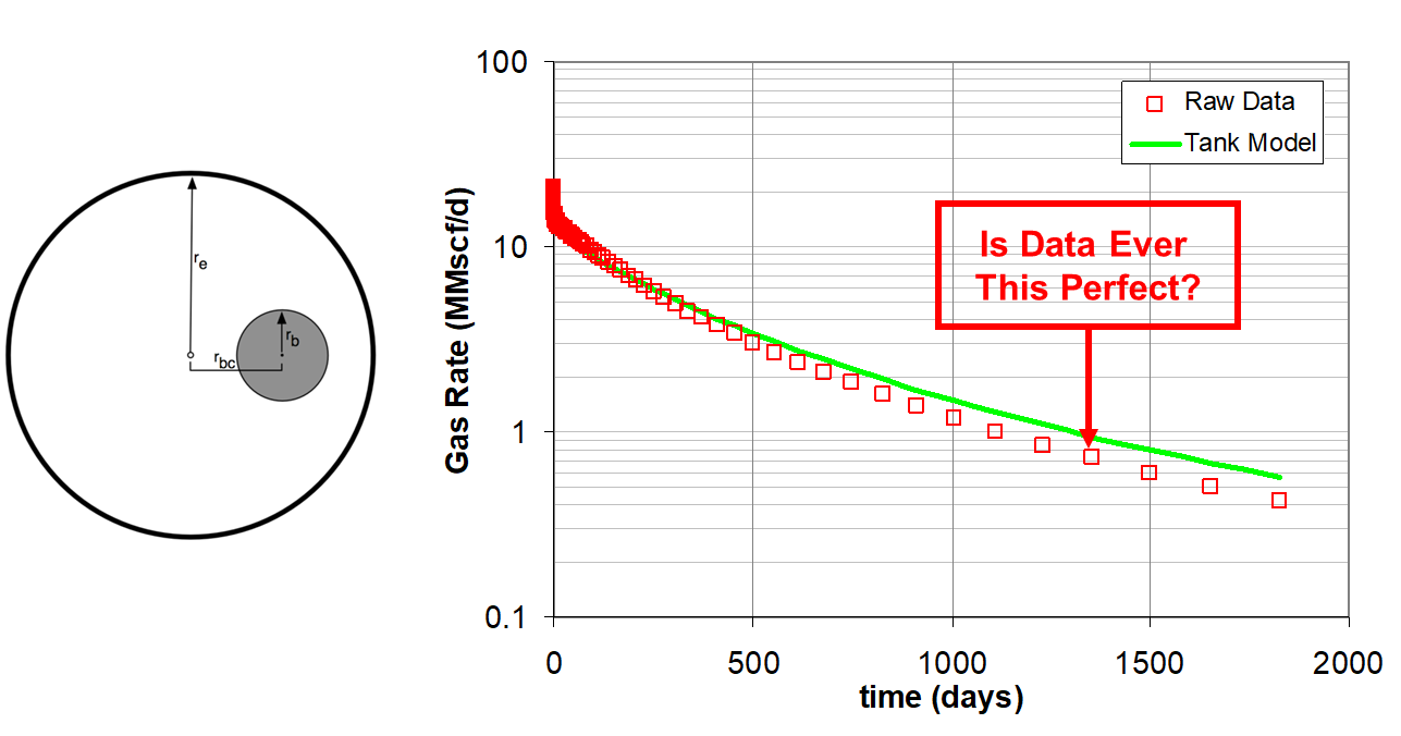
In this example, a reservoir was simulated with an internal no-flow boundary (a 72 Acre region with zero permeability) within a larger 640 Acre reservoir of 20 md, and 5.5 Bcf of gas. Flowing material balance analysis produced an equivalent reservoir of 16.5 md, with a OGIP of 5.4 Bcf. The net area calculated (using the volumetric parameters such as net pay, porosity, and more) was 567 Acre (which closely approximates 568 = 640-72). Production based analysis produced the equivalent reservoir which:
-
Will produce reliable results for physics based forecasting honouring effective productivity index, and material balance.
-
Not necessarily great for reservoir characterization.
Numerical Simulation Example
In this example, we generate a numerical model with the following criteria:
|
Parameter |
Single Phase Vertical Well |
|---|---|
|
Area (Square) |
10,000 x 10,000 ft |
|
Permeability. |
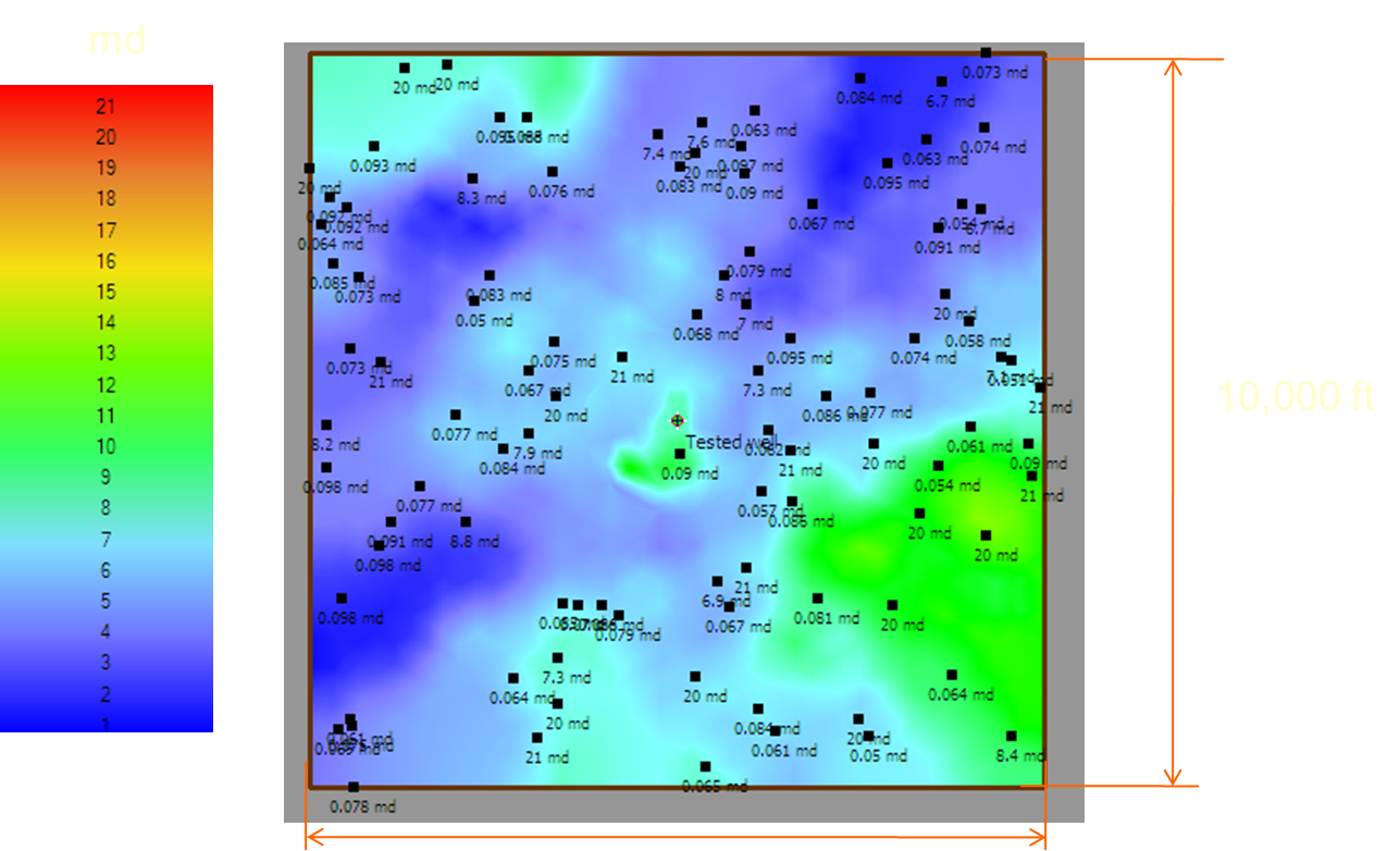
0.05 - 21 md (Average = 5.31 md) Permeability field was generated using a uniform distribution generator |
|
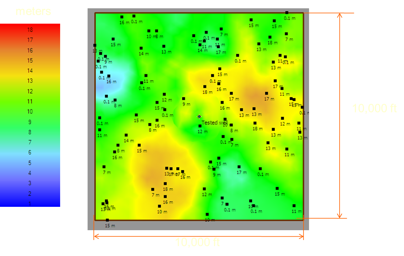
Net Pay |
0.1 - 18 m (Average = 10.1 m, or 32.8 ft) Net pay field was generated using a uniform distribution generator |
|
Porosity |
10% |
|
Initial Pressure |
5,000 psia |
|
Water Saturation |
0 |
|
Gas Gravity |
0.7 Dim |
|
OGIP |
87.2 Bcf (numerically calculated) |
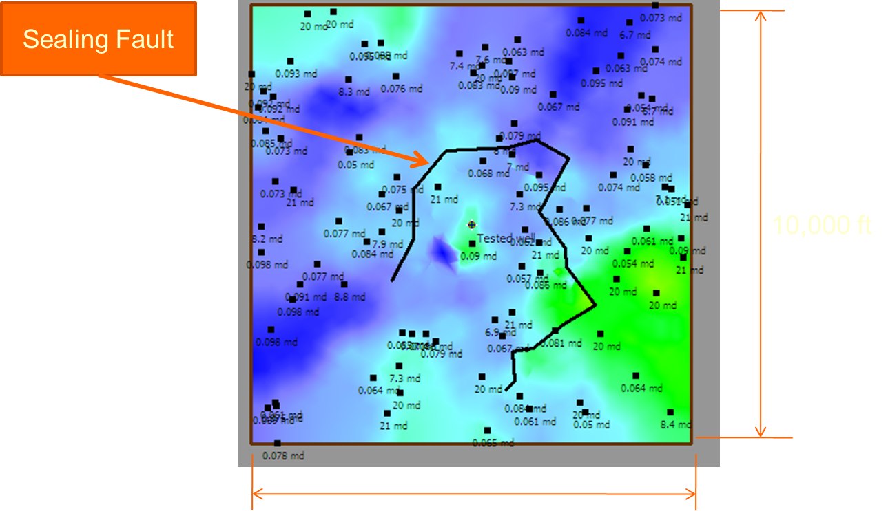
Graphical representations of the random permeability and net pay field are shown below:
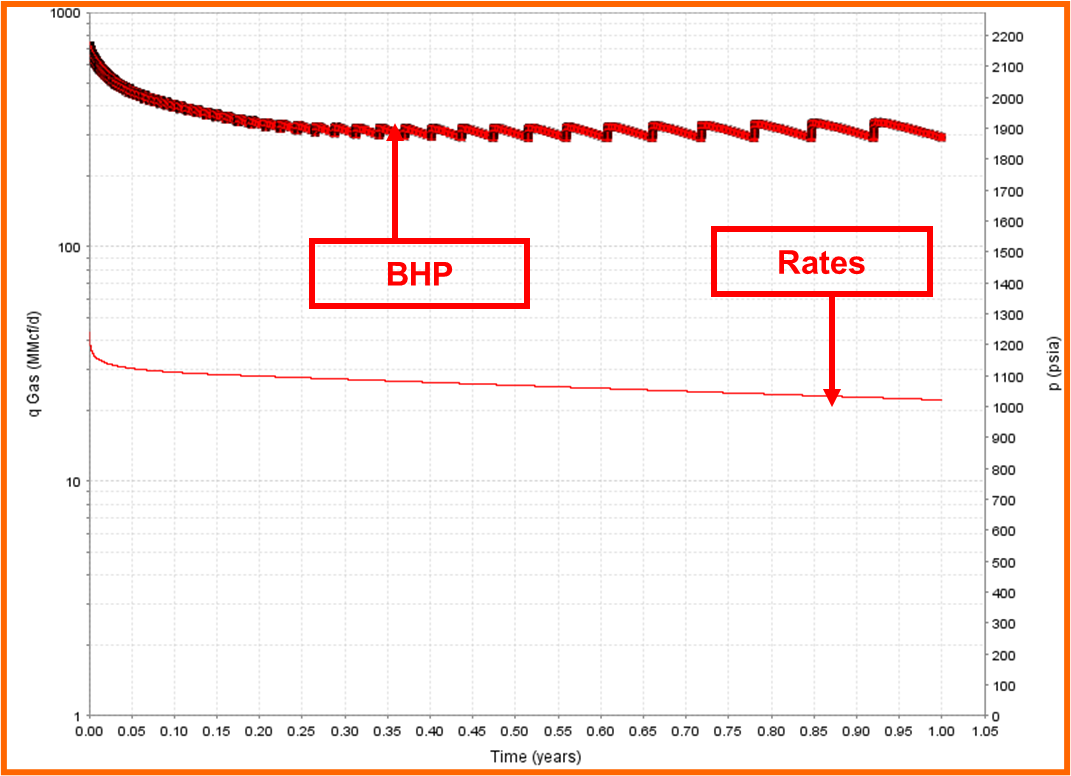
Using the numerical model, a production forecast was generated with a slightly varying BHP, ranging from nearly 2,500 psia to a somewhat stable value of about 1,900 psia - a relatively large drawdown compared to the initial pressure of 5,000 psia.
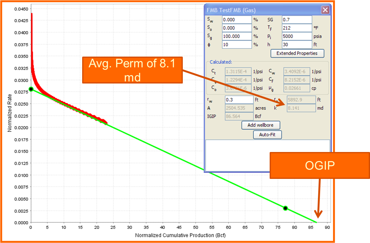
The Flowing Material Balance (or FMB) for the simulated example is shown below. As can be seen, the FMB produced the following results:
|
Parameter |
FMB |
Simulator |
|---|---|---|
|
Average Permeability |
8.141 md |
0.05 - 21 md (Average = 5.31 md) |
|
OGIP (or IGIP) |
86.6 Bcf |
87.2 Bcf |
|
Drainage Area |
2504 Acres |
2295 Acres (10,000 x 10,000 ft) |
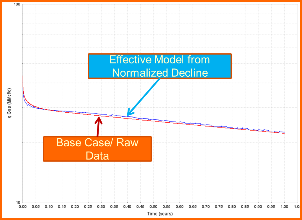
Given that the FMB assumes a constant net pay of 30 ft, the total effective drainage area will not be similar to the numerical model - but nonetheless, it is a close approximation. We do know that the FMB will provide the correct productivity index; thus comparing the production forecasts (from transient to PSS condition), we find excellent correlation
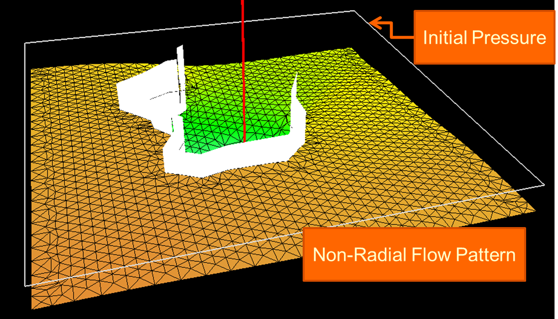
Numerical Simulation Example: Introduction of No-Flow Boundary
Following on the previous discussion, an arbitrary shaped no-flow boundary was introduced into the simulator (all other parameters remained the same). Also shown in the pressure contour for the system (at an arbitrary time) we have a none-radial, none symmetrical flow pattern.
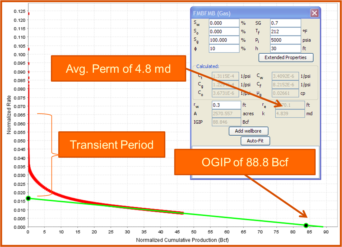
The FMB, as well as a traditional PTA analysis shown below.
-
The FMB suggests an effective permeability of 4.8 md with an effective drainage area of 2570 Acres, and OGIP of 88.8 Bcf.
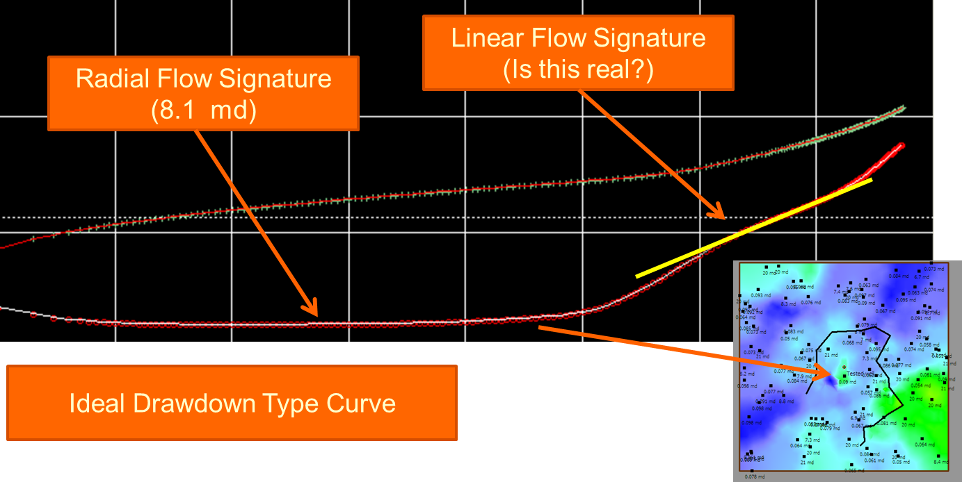
-
The PTA suggests an average reservoir permeability of 8.1 md, with late-time PSS shown past “apparent“ radial flow.
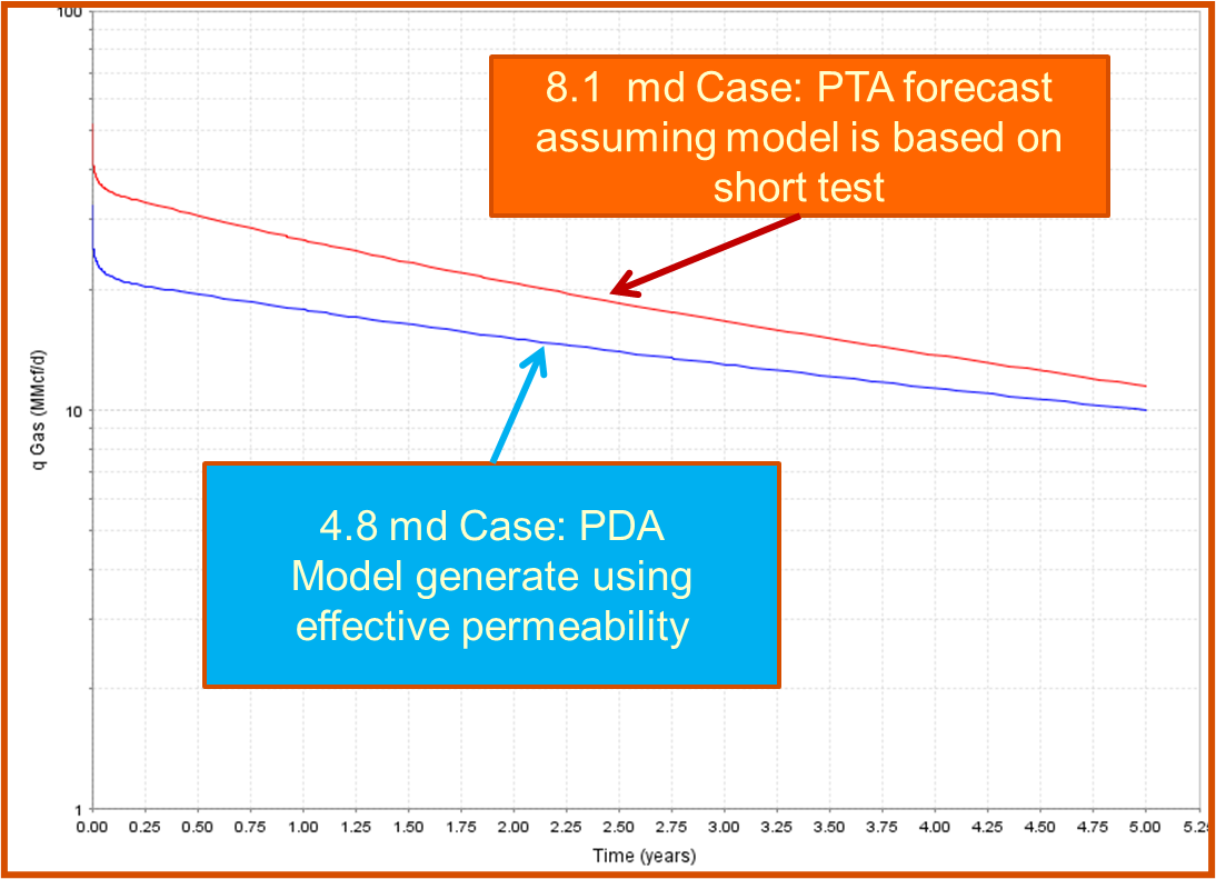
-
A production forecast using both FMB/PTA results shows radically different results.
|
FMB |
PTA Analysis |
|---|---|
|
|
|
References:
-
T. A. Blasingame “Drowning In Data — The Future of Reservoir Performance Analysis”
-
D. Ilk, and T. A. Blasingame “Forecasting: Forecasting Future Performance for Various Production/ Completion/ Development Scenarios”, PETE 612, Unconventional Oil and Reservoirs, 2018.
-
Colin Lyle Jordan, Robert Jackson, Short Course: Complex Well Analyses & Reservoir Engineering Methods for Unconventional Gas, 11th Annual Unconventional Gas Conference, November 20, 2009.
-
Abraham Sageev, Pressure Transient Analysis of Reservoirs With Linear or Internal Circular Boundaries, Stanford Geothermal Program Interdisciplinary Research, SGP-TR-65.
-
Helge H. Haldorsen, Simulator Parameter Assignment and the Problem of Scale in Reservoir Engineering, Reservoir Characterization Journal, 1986