
The following section provides some background on basic methodologies used for constructing type wells. These approaches are designed to generate representative type curves by leveraging historical production data, statistical techniques, and decline analysis. Each method has its own strengths, limitations, and assumptions, which should be carefully considered when selecting the most appropriate approach for a given development scenario.
Time Slice (TS) Method
The Time Slice method is a common way to build probability-based type curves, and it's the one used in most commercial software.
Here's how it works:
-
For each production month, take the production rates from all wells that have data for that month.
-
Sort the rates from highest to lowest.
-
Pick the value at the desired percentile — for example, the P50 (median), P10, or P90 — and use that as the production rate for that month.
-
Repeat this process for every month where enough wells still have data.
Once the number of wells with data drops below a certain threshold (usually 75% of the original well count), the data is considered too sparse. At that point, you stop using historical data and complete the rest of the curve using decline analysis (like exponential or hyperbolic decline models).
Limitation for TS Method
According to the literature, the limitations include:
-
Fewer Wells Over Time: As production time increases, fewer wells have available data, especially after a certain point (like when only 75% of the wells still have data). This can cause inaccuracies in the results.
-
Affected by Outliers: The TS method ranks and picks rates month by month. This means that outliers (extremely high or low values) can distort the results, especially when there are not many wells left in later months.
-
Doesn't Reflect Real Decline Patterns: Since the TS method picks different wells each month, it doesn’t show the actual decline curve of a single well. Instead, it combines rates from different wells, which doesn’t reflect how a real well would behave.
-
Problems When Curves Cross: If the production profiles of wells cross over one another (where a higher-rate well later becomes a lower-rate well), this method doesn’t handle it well, leading to inaccurate results. This is a major issue in the TS method (Russell and Freeborn, 2013).
-
Doesn't Match EUR: The TS method doesn’t focus on the EUR of each well. The final type curve doesn’t represent a real well’s EUR, which makes it harder to link to specific real-world wells.
-
May Lose Consistency in Data: If the number of wells gets too small or uneven (especially after using 75% of available data), the method may not be consistent anymore, leading to even more inaccurate results.
-
Doesn't Capture Individual Well Behaviour: The method doesn’t track how each individual well behaves. It just takes an average from a variety of wells, so the final curve doesn't represent the specific behaviour of any one well.
Monte Carlo-Based Aggregation Method
Aggregation is the process of combining production data from multiple wells to construct a type well or type curve that represents the performance of a group of similar wells (Freeborn and Russell 2016).
Key Aggregation Principles
-
Use Forecasted EURs: Estimate the EUR of each well using a consistent method (e.g., 3 years of production data fitted with a modified hyperbolic decline model and a 5% terminal decline rate).
-
Be Cautious of Bias: Be aware that using a fixed terminal decline rate (e.g., 5%) can introduce bias, particularly if it's not accurate for all wells.
-
Minimise Errors Through Aggregation: When aggregating EURs from multiple wells, random errors tend to cancel out, improving the reliability of the overall EUR distribution.
-
Avoid Time-Slice Weaknesses: Methods like the TS approach can lead to inaccurate type wells when production profiles cross or behave differently over time.
-
Use Representative Data Only: The aggregated data should represent the wells planned for future drilling, both in geology (reservoir quality) and operational practices (completion methods).
Guidelines for Selecting Representative Wells
-
Match Reservoir and Completion: Select wells that have similar reservoir properties (e.g., rock type, pressure) and completion techniques (e.g., fracture stimulation, lateral length) as those intended for future drilling.
-
Do Not Mix Operator Performance Levels: Avoid mixing wells from operators with different performance levels. For instance, don't use data from a top-performing (1st decile) operator if your wells are expected to perform at a lower (3rd quartile) level.
-
Adjust Profiles If Needed: If you don’t have enough data, you may include additional wells, but you must scale or adjust their rate/time profiles to make them representative of the planned wells.
-
Use Consistent Decline Analysis: Apply the same decline method (e.g., modified hyperbolic with 5% terminal decline) across all selected wells to ensure consistency.
-
Avoid Crossed Production Profiles: Be cautious of wells whose production curves cross one another, as this can confuse the aggregation process and lead to unreliable type curves.
A Step-by-Step Process to Create Aggregated Type Wells
Step 1: Build the EUR Probability Distribution
-
Estimate EURs for All Wells
Begin with a set of N wells for which production data is available. For each well, estimate its Estimated Ultimate Recovery (EUR) using a consistent decline curve model — typically a modified hyperbolic model with a 5% nominal terminal decline rate. -
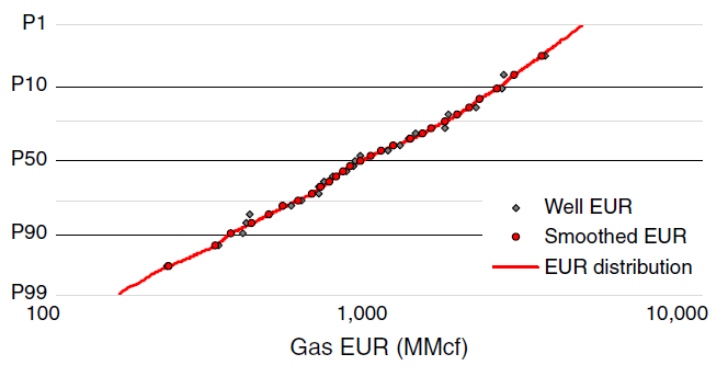
Generate the EUR Distribution
After estimating EURs for all wells, compile them into a probability distribution. In most cases, this distribution tends to follow a log-normal shape due to the nature of production variability. -
Smooth the EUR Distribution (Optional but Recommended)
To reduce noise and remove local anomalies, apply a sliding-window smoothing technique:-
Use a 7-point moving window across the sorted EUR values.
-
For each window, fit a log-normal curve.
-
Replace the middle point (4th value) with the fitted curve’s predicted value.
-
Slide the window forward by one position and repeat the process.
-
For the edges of the dataset, use 5-point or 3-point windows to avoid data loss.
-
This process creates a cleaner, more reliable EUR probability distribution for simulation.
Step 2: Monte Carlo Simulation for Aggregated EUR
-
Define Simulation Parameters
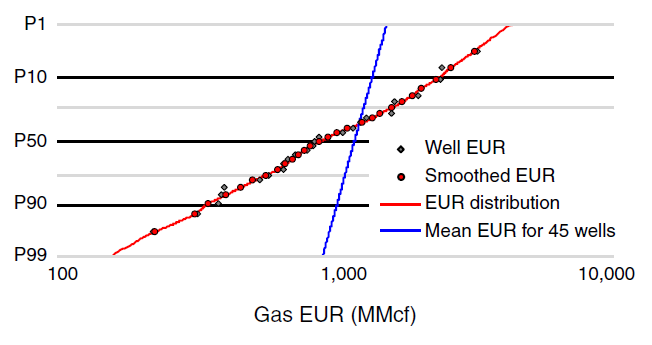
Choose the number of wells to simulate per trial (e.g., 45 wells), and the total number of trials (e.g., 25,000). The more trials you run, the more robust your aggregated results will be. -
Run Simulations
For each trial:-
Randomly select 45 percentile values between 0.1% and 99.9%.
-
Use your smoothed EUR distribution to convert each percentile into an EUR value.
-
Calculate the mean EUR of the selected values for that trial.
-
Store this mean EUR.
-
-
Build the Aggregated EUR Distribution
After thousands of trials, the resulting set of average EURs forms the aggregated EUR probability distribution — representing the expected performance of future drilling programs based on your well dataset.
Step 3: Determine Well Weighting Factors By Running Additional Monte Carlo Trials
To generate a final aggregated type well, we calculate weighting factors for each individual well which were using in the step 1 to create smoothed EUR probability distribution. These factors represent the relative importance or likelihood of each well being part of a forecast, based on successful simulation outcomes.
Here’s the step-by-step process:
-
Identify Successful Trials
Define a target EUR value (e.g., P90 = 1,010 MMcf), and select a narrow range around it (e.g., 1,009.9 to 1,010.1 MMcf).
A trial is "successful" if the mean EUR for that trial falls within this range. -
Track Well Appearances in Successful Trials
For each successful trial, record how often each well’s EUR (or a bracketing combination) was selected. -
Bracket EURs (When Needed)
-
If the simulated EUR falls between two known well EURs, distribute the count proportionally between them.
-
If the simulated EUR is outside the known range, assign a scaled value to the nearest extreme well using a ratio (e.g., simulated EUR ÷ closest well EUR).
Example:
If a simulated EUR is 800 MMcf and falls between:-
Well A: 791 MMcf
-
Well B: 836 MMcf
Then: -
Well A gets 80% of the tally
-
Well B gets 20%
-
-
Calculate Weighting Factors
After processing all successful trials:-
Sum the tallies for each well.
-
Divide each well’s tally by the total tally across all wells:
-
' aria-hidden='true'%3e %3cg transform='translate(167%2c0)'%3e %3cg transform='translate(-11%2c0)'%3e %3cg transform='translate(0%2c45)'%3e %3cuse xlink:href='%23E1-MJMAIN-57'%3e%3c/use%3e %3cuse xlink:href='%23E1-MJMAIN-65' x='1028' y='0'%3e%3c/use%3e %3cuse xlink:href='%23E1-MJMAIN-69' x='1473' y='0'%3e%3c/use%3e %3cuse xlink:href='%23E1-MJMAIN-67' x='1751' y='0'%3e%3c/use%3e %3cuse xlink:href='%23E1-MJMAIN-68' x='2252' y='0'%3e%3c/use%3e %3cuse xlink:href='%23E1-MJMAIN-74' x='2808' y='0'%3e%3c/use%3e %3cuse xlink:href='%23E1-MJMAIN-69' x='3198' y='0'%3e%3c/use%3e %3cuse xlink:href='%23E1-MJMAIN-6E' x='3476' y='0'%3e%3c/use%3e %3cuse xlink:href='%23E1-MJMAIN-67' x='4033' y='0'%3e%3c/use%3e %3cuse xlink:href='%23E1-MJMAIN-46' x='4783' y='0'%3e%3c/use%3e %3cuse xlink:href='%23E1-MJMAIN-61' x='5437' y='0'%3e%3c/use%3e %3cuse xlink:href='%23E1-MJMAIN-63' x='5937' y='0'%3e%3c/use%3e %3cuse xlink:href='%23E1-MJMAIN-74' x='6382' y='0'%3e%3c/use%3e %3cuse xlink:href='%23E1-MJMAIN-6F' x='6771' y='0'%3e%3c/use%3e %3cuse xlink:href='%23E1-MJMAIN-72' x='7272' y='0'%3e%3c/use%3e %3cuse xlink:href='%23E1-MJMAIN-66' x='7914' y='0'%3e%3c/use%3e %3cuse xlink:href='%23E1-MJMAIN-6F' x='8221' y='0'%3e%3c/use%3e %3cuse xlink:href='%23E1-MJMAIN-72' x='8721' y='0'%3e%3c/use%3e %3cuse xlink:href='%23E1-MJMAIN-57' x='9364' y='0'%3e%3c/use%3e %3cuse xlink:href='%23E1-MJMAIN-65' x='10392' y='0'%3e%3c/use%3e %3cuse xlink:href='%23E1-MJMAIN-6C' x='10837' y='0'%3e%3c/use%3e %3cuse xlink:href='%23E1-MJMAIN-6C' x='11115' y='0'%3e%3c/use%3e %3cuse xlink:href='%23E1-MJMATHI-58' x='11644' y='0'%3e%3c/use%3e %3cuse xlink:href='%23E1-MJMAIN-3D' x='12774' y='0'%3e%3c/use%3e %3cg transform='translate(13552%2c0)'%3e %3cg transform='translate(397%2c0)'%3e %3crect stroke='none' width='7260' height='60' x='0' y='220'%3e%3c/rect%3e %3cg transform='translate(60%2c724)'%3e %3cuse xlink:href='%23E1-MJMAIN-54'%3e%3c/use%3e %3cuse xlink:href='%23E1-MJMAIN-61' x='722' y='0'%3e%3c/use%3e %3cuse xlink:href='%23E1-MJMAIN-6C' x='1223' y='0'%3e%3c/use%3e %3cuse xlink:href='%23E1-MJMAIN-6C' x='1501' y='0'%3e%3c/use%3e %3cuse xlink:href='%23E1-MJMAIN-79' x='1780' y='0'%3e%3c/use%3e %3cuse xlink:href='%23E1-MJMAIN-66' x='2558' y='0'%3e%3c/use%3e %3cuse xlink:href='%23E1-MJMAIN-6F' x='2865' y='0'%3e%3c/use%3e %3cuse xlink:href='%23E1-MJMAIN-72' x='3365' y='0'%3e%3c/use%3e %3cuse xlink:href='%23E1-MJMAIN-57' x='4008' y='0'%3e%3c/use%3e %3cuse xlink:href='%23E1-MJMAIN-65' x='5036' y='0'%3e%3c/use%3e %3cuse xlink:href='%23E1-MJMAIN-6C' x='5481' y='0'%3e%3c/use%3e %3cuse xlink:href='%23E1-MJMAIN-6C' x='5759' y='0'%3e%3c/use%3e %3cuse xlink:href='%23E1-MJMATHI-58' x='6288' y='0'%3e%3c/use%3e %3c/g%3e %3cg transform='translate(791%2c-771)'%3e %3cuse xlink:href='%23E1-MJSZ1-2211' x='0' y='0'%3e%3c/use%3e %3cg transform='translate(1223%2c0)'%3e %3cuse xlink:href='%23E1-MJMAIN-41'%3e%3c/use%3e %3cuse xlink:href='%23E1-MJMAIN-6C' x='750' y='0'%3e%3c/use%3e %3cuse xlink:href='%23E1-MJMAIN-6C' x='1029' y='0'%3e%3c/use%3e %3cuse xlink:href='%23E1-MJMAIN-54' x='1557' y='0'%3e%3c/use%3e %3cuse xlink:href='%23E1-MJMAIN-61' x='2280' y='0'%3e%3c/use%3e %3cuse xlink:href='%23E1-MJMAIN-6C' x='2780' y='0'%3e%3c/use%3e %3cuse xlink:href='%23E1-MJMAIN-6C' x='3059' y='0'%3e%3c/use%3e %3cuse xlink:href='%23E1-MJMAIN-69' x='3337' y='0'%3e%3c/use%3e %3cuse xlink:href='%23E1-MJMAIN-65' x='3616' y='0'%3e%3c/use%3e %3cuse xlink:href='%23E1-MJMAIN-73' x='4060' y='0'%3e%3c/use%3e %3c/g%3e %3c/g%3e %3c/g%3e %3c/g%3e %3c/g%3e %3c/g%3e %3c/g%3e %3c/g%3e %3c/svg%3e)
These factors indicate how representative each well is in successful outcomes.
Step 4: Construct the Final Aggregated Type Well
Multiply each well’s production rate/time profile (historical and forecast) by its weighting factor, then sum the results across all wells:
%5cend%7barray%7d%3c/title%3e %3cdefs aria-hidden='true'%3e %3cpath stroke-width='1' id='E1-MJMAIN-41' d='M255 0Q240 3 140 3Q48 3 39 0H32V46H47Q119 49 139 88Q140 91 192 245T295 553T348 708Q351 716 366 716H376Q396 715 400 709Q402 707 508 390L617 67Q624 54 636 51T687 46H717V0H708Q699 3 581 3Q458 3 437 0H427V46H440Q510 46 510 64Q510 66 486 138L462 209H229L209 150Q189 91 189 85Q189 72 209 59T259 46H264V0H255ZM447 255L345 557L244 256Q244 255 345 255H447Z'%3e%3c/path%3e %3cpath stroke-width='1' id='E1-MJMAIN-67' d='M329 409Q373 453 429 453Q459 453 472 434T485 396Q485 382 476 371T449 360Q416 360 412 390Q410 404 415 411Q415 412 416 414V415Q388 412 363 393Q355 388 355 386Q355 385 359 381T368 369T379 351T388 325T392 292Q392 230 343 187T222 143Q172 143 123 171Q112 153 112 133Q112 98 138 81Q147 75 155 75T227 73Q311 72 335 67Q396 58 431 26Q470 -13 470 -72Q470 -139 392 -175Q332 -206 250 -206Q167 -206 107 -175Q29 -140 29 -75Q29 -39 50 -15T92 18L103 24Q67 55 67 108Q67 155 96 193Q52 237 52 292Q52 355 102 398T223 442Q274 442 318 416L329 409ZM299 343Q294 371 273 387T221 404Q192 404 171 388T145 343Q142 326 142 292Q142 248 149 227T179 192Q196 182 222 182Q244 182 260 189T283 207T294 227T299 242Q302 258 302 292T299 343ZM403 -75Q403 -50 389 -34T348 -11T299 -2T245 0H218Q151 0 138 -6Q118 -15 107 -34T95 -74Q95 -84 101 -97T122 -127T170 -155T250 -167Q319 -167 361 -139T403 -75Z'%3e%3c/path%3e %3cpath stroke-width='1' id='E1-MJMAIN-72' d='M36 46H50Q89 46 97 60V68Q97 77 97 91T98 122T98 161T98 203Q98 234 98 269T98 328L97 351Q94 370 83 376T38 385H20V408Q20 431 22 431L32 432Q42 433 60 434T96 436Q112 437 131 438T160 441T171 442H174V373Q213 441 271 441H277Q322 441 343 419T364 373Q364 352 351 337T313 322Q288 322 276 338T263 372Q263 381 265 388T270 400T273 405Q271 407 250 401Q234 393 226 386Q179 341 179 207V154Q179 141 179 127T179 101T180 81T180 66V61Q181 59 183 57T188 54T193 51T200 49T207 48T216 47T225 47T235 46T245 46H276V0H267Q249 3 140 3Q37 3 28 0H20V46H36Z'%3e%3c/path%3e %3cpath stroke-width='1' id='E1-MJMAIN-65' d='M28 218Q28 273 48 318T98 391T163 433T229 448Q282 448 320 430T378 380T406 316T415 245Q415 238 408 231H126V216Q126 68 226 36Q246 30 270 30Q312 30 342 62Q359 79 369 104L379 128Q382 131 395 131H398Q415 131 415 121Q415 117 412 108Q393 53 349 21T250 -11Q155 -11 92 58T28 218ZM333 275Q322 403 238 411H236Q228 411 220 410T195 402T166 381T143 340T127 274V267H333V275Z'%3e%3c/path%3e %3cpath stroke-width='1' id='E1-MJMAIN-61' d='M137 305T115 305T78 320T63 359Q63 394 97 421T218 448Q291 448 336 416T396 340Q401 326 401 309T402 194V124Q402 76 407 58T428 40Q443 40 448 56T453 109V145H493V106Q492 66 490 59Q481 29 455 12T400 -6T353 12T329 54V58L327 55Q325 52 322 49T314 40T302 29T287 17T269 6T247 -2T221 -8T190 -11Q130 -11 82 20T34 107Q34 128 41 147T68 188T116 225T194 253T304 268H318V290Q318 324 312 340Q290 411 215 411Q197 411 181 410T156 406T148 403Q170 388 170 359Q170 334 154 320ZM126 106Q126 75 150 51T209 26Q247 26 276 49T315 109Q317 116 318 175Q318 233 317 233Q309 233 296 232T251 223T193 203T147 166T126 106Z'%3e%3c/path%3e %3cpath stroke-width='1' id='E1-MJMAIN-74' d='M27 422Q80 426 109 478T141 600V615H181V431H316V385H181V241Q182 116 182 100T189 68Q203 29 238 29Q282 29 292 100Q293 108 293 146V181H333V146V134Q333 57 291 17Q264 -10 221 -10Q187 -10 162 2T124 33T105 68T98 100Q97 107 97 248V385H18V422H27Z'%3e%3c/path%3e %3cpath stroke-width='1' id='E1-MJMAIN-64' d='M376 495Q376 511 376 535T377 568Q377 613 367 624T316 637H298V660Q298 683 300 683L310 684Q320 685 339 686T376 688Q393 689 413 690T443 693T454 694H457V390Q457 84 458 81Q461 61 472 55T517 46H535V0Q533 0 459 -5T380 -11H373V44L365 37Q307 -11 235 -11Q158 -11 96 50T34 215Q34 315 97 378T244 442Q319 442 376 393V495ZM373 342Q328 405 260 405Q211 405 173 369Q146 341 139 305T131 211Q131 155 138 120T173 59Q203 26 251 26Q322 26 373 103V342Z'%3e%3c/path%3e %3cpath stroke-width='1' id='E1-MJMAIN-54' d='M36 443Q37 448 46 558T55 671V677H666V671Q667 666 676 556T685 443V437H645V443Q645 445 642 478T631 544T610 593Q593 614 555 625Q534 630 478 630H451H443Q417 630 414 618Q413 616 413 339V63Q420 53 439 50T528 46H558V0H545L361 3Q186 1 177 0H164V46H194Q264 46 283 49T309 63V339V550Q309 620 304 625T271 630H244H224Q154 630 119 601Q101 585 93 554T81 486T76 443V437H36V443Z'%3e%3c/path%3e %3cpath stroke-width='1' id='E1-MJMAIN-79' d='M69 -66Q91 -66 104 -80T118 -116Q118 -134 109 -145T91 -160Q84 -163 97 -166Q104 -168 111 -168Q131 -168 148 -159T175 -138T197 -106T213 -75T225 -43L242 0L170 183Q150 233 125 297Q101 358 96 368T80 381Q79 382 78 382Q66 385 34 385H19V431H26L46 430Q65 430 88 429T122 428Q129 428 142 428T171 429T200 430T224 430L233 431H241V385H232Q183 385 185 366L286 112Q286 113 332 227L376 341V350Q376 365 366 373T348 383T334 385H331V431H337H344Q351 431 361 431T382 430T405 429T422 429Q477 429 503 431H508V385H497Q441 380 422 345Q420 343 378 235T289 9T227 -131Q180 -204 113 -204Q69 -204 44 -177T19 -116Q19 -89 35 -78T69 -66Z'%3e%3c/path%3e %3cpath stroke-width='1' id='E1-MJMAIN-70' d='M36 -148H50Q89 -148 97 -134V-126Q97 -119 97 -107T97 -77T98 -38T98 6T98 55T98 106Q98 140 98 177T98 243T98 296T97 335T97 351Q94 370 83 376T38 385H20V408Q20 431 22 431L32 432Q42 433 61 434T98 436Q115 437 135 438T165 441T176 442H179V416L180 390L188 397Q247 441 326 441Q407 441 464 377T522 216Q522 115 457 52T310 -11Q242 -11 190 33L182 40V-45V-101Q182 -128 184 -134T195 -145Q216 -148 244 -148H260V-194H252L228 -193Q205 -192 178 -192T140 -191Q37 -191 28 -194H20V-148H36ZM424 218Q424 292 390 347T305 402Q234 402 182 337V98Q222 26 294 26Q345 26 384 80T424 218Z'%3e%3c/path%3e %3cpath stroke-width='1' id='E1-MJMAIN-57' d='M792 683Q810 680 914 680Q991 680 1003 683H1009V637H996Q931 633 915 598Q912 591 863 438T766 135T716 -17Q711 -22 694 -22Q676 -22 673 -15Q671 -13 593 231L514 477L435 234Q416 174 391 92T358 -6T341 -22H331Q314 -21 310 -15Q309 -14 208 302T104 622Q98 632 87 633Q73 637 35 637H18V683H27Q69 681 154 681Q164 681 181 681T216 681T249 682T276 683H287H298V637H285Q213 637 213 620Q213 616 289 381L364 144L427 339Q490 535 492 546Q487 560 482 578T475 602T468 618T461 628T449 633T433 636T408 637H380V683H388Q397 680 508 680Q629 680 650 683H660V637H647Q576 637 576 619L727 146Q869 580 869 600Q869 605 863 612T839 627T794 637H783V683H792Z'%3e%3c/path%3e %3cpath stroke-width='1' id='E1-MJMAIN-6C' d='M42 46H56Q95 46 103 60V68Q103 77 103 91T103 124T104 167T104 217T104 272T104 329Q104 366 104 407T104 482T104 542T103 586T103 603Q100 622 89 628T44 637H26V660Q26 683 28 683L38 684Q48 685 67 686T104 688Q121 689 141 690T171 693T182 694H185V379Q185 62 186 60Q190 52 198 49Q219 46 247 46H263V0H255L232 1Q209 2 183 2T145 3T107 3T57 1L34 0H26V46H42Z'%3e%3c/path%3e %3cpath stroke-width='1' id='E1-MJMAIN-3D' d='M56 347Q56 360 70 367H707Q722 359 722 347Q722 336 708 328L390 327H72Q56 332 56 347ZM56 153Q56 168 72 173H708Q722 163 722 153Q722 140 707 133H70Q56 140 56 153Z'%3e%3c/path%3e %3cpath stroke-width='1' id='E1-MJSZ2-2211' d='M60 948Q63 950 665 950H1267L1325 815Q1384 677 1388 669H1348L1341 683Q1320 724 1285 761Q1235 809 1174 838T1033 881T882 898T699 902H574H543H251L259 891Q722 258 724 252Q725 250 724 246Q721 243 460 -56L196 -356Q196 -357 407 -357Q459 -357 548 -357T676 -358Q812 -358 896 -353T1063 -332T1204 -283T1307 -196Q1328 -170 1348 -124H1388Q1388 -125 1381 -145T1356 -210T1325 -294L1267 -449L666 -450Q64 -450 61 -448Q55 -446 55 -439Q55 -437 57 -433L590 177Q590 178 557 222T452 366T322 544L56 909L55 924Q55 945 60 948Z'%3e%3c/path%3e %3cpath stroke-width='1' id='E1-MJMATHI-69' d='M184 600Q184 624 203 642T247 661Q265 661 277 649T290 619Q290 596 270 577T226 557Q211 557 198 567T184 600ZM21 287Q21 295 30 318T54 369T98 420T158 442Q197 442 223 419T250 357Q250 340 236 301T196 196T154 83Q149 61 149 51Q149 26 166 26Q175 26 185 29T208 43T235 78T260 137Q263 149 265 151T282 153Q302 153 302 143Q302 135 293 112T268 61T223 11T161 -11Q129 -11 102 10T74 74Q74 91 79 106T122 220Q160 321 166 341T173 380Q173 404 156 404H154Q124 404 99 371T61 287Q60 286 59 284T58 281T56 279T53 278T49 278T41 278H27Q21 284 21 287Z'%3e%3c/path%3e %3cpath stroke-width='1' id='E1-MJMAIN-28' d='M94 250Q94 319 104 381T127 488T164 576T202 643T244 695T277 729T302 750H315H319Q333 750 333 741Q333 738 316 720T275 667T226 581T184 443T167 250T184 58T225 -81T274 -167T316 -220T333 -241Q333 -250 318 -250H315H302L274 -226Q180 -141 137 -14T94 250Z'%3e%3c/path%3e %3cpath stroke-width='1' id='E1-MJMAIN-69' d='M69 609Q69 637 87 653T131 669Q154 667 171 652T188 609Q188 579 171 564T129 549Q104 549 87 564T69 609ZM247 0Q232 3 143 3Q132 3 106 3T56 1L34 0H26V46H42Q70 46 91 49Q100 53 102 60T104 102V205V293Q104 345 102 359T88 378Q74 385 41 385H30V408Q30 431 32 431L42 432Q52 433 70 434T106 436Q123 437 142 438T171 441T182 442H185V62Q190 52 197 50T232 46H255V0H247Z'%3e%3c/path%3e %3cpath stroke-width='1' id='E1-MJMAIN-68' d='M41 46H55Q94 46 102 60V68Q102 77 102 91T102 124T102 167T103 217T103 272T103 329Q103 366 103 407T103 482T102 542T102 586T102 603Q99 622 88 628T43 637H25V660Q25 683 27 683L37 684Q47 685 66 686T103 688Q120 689 140 690T170 693T181 694H184V367Q244 442 328 442Q451 442 463 329Q464 322 464 190V104Q464 66 466 59T477 49Q498 46 526 46H542V0H534L510 1Q487 2 460 2T422 3Q319 3 310 0H302V46H318Q379 46 379 62Q380 64 380 200Q379 335 378 343Q372 371 358 385T334 402T308 404Q263 404 229 370Q202 343 195 315T187 232V168V108Q187 78 188 68T191 55T200 49Q221 46 249 46H265V0H257L234 1Q210 2 183 2T145 3Q42 3 33 0H25V46H41Z'%3e%3c/path%3e %3cpath stroke-width='1' id='E1-MJMAIN-6E' d='M41 46H55Q94 46 102 60V68Q102 77 102 91T102 122T103 161T103 203Q103 234 103 269T102 328V351Q99 370 88 376T43 385H25V408Q25 431 27 431L37 432Q47 433 65 434T102 436Q119 437 138 438T167 441T178 442H181V402Q181 364 182 364T187 369T199 384T218 402T247 421T285 437Q305 442 336 442Q450 438 463 329Q464 322 464 190V104Q464 66 466 59T477 49Q498 46 526 46H542V0H534L510 1Q487 2 460 2T422 3Q319 3 310 0H302V46H318Q379 46 379 62Q380 64 380 200Q379 335 378 343Q372 371 358 385T334 402T308 404Q263 404 229 370Q202 343 195 315T187 232V168V108Q187 78 188 68T191 55T200 49Q221 46 249 46H265V0H257L234 1Q210 2 183 2T145 3Q42 3 33 0H25V46H41Z'%3e%3c/path%3e %3cpath stroke-width='1' id='E1-MJMAIN-46' d='M128 619Q121 626 117 628T101 631T58 634H25V680H582V676Q584 670 596 560T610 444V440H570V444Q563 493 561 501Q555 538 543 563T516 601T477 622T431 631T374 633H334H286Q252 633 244 631T233 621Q232 619 232 490V363H284Q287 363 303 363T327 364T349 367T372 373T389 385Q407 403 410 459V480H450V200H410V221Q407 276 389 296Q381 303 371 307T348 313T327 316T303 317T284 317H232V189L233 61Q240 54 245 52T270 48T333 46H360V0H348Q324 3 182 3Q51 3 36 0H25V46H58Q100 47 109 49T128 61V619Z'%3e%3c/path%3e %3cpath stroke-width='1' id='E1-MJMAIN-63' d='M370 305T349 305T313 320T297 358Q297 381 312 396Q317 401 317 402T307 404Q281 408 258 408Q209 408 178 376Q131 329 131 219Q131 137 162 90Q203 29 272 29Q313 29 338 55T374 117Q376 125 379 127T395 129H409Q415 123 415 120Q415 116 411 104T395 71T366 33T318 2T249 -11Q163 -11 99 53T34 214Q34 318 99 383T250 448T370 421T404 357Q404 334 387 320Z'%3e%3c/path%3e %3cpath stroke-width='1' id='E1-MJMAIN-6F' d='M28 214Q28 309 93 378T250 448Q340 448 405 380T471 215Q471 120 407 55T250 -10Q153 -10 91 57T28 214ZM250 30Q372 30 372 193V225V250Q372 272 371 288T364 326T348 362T317 390T268 410Q263 411 252 411Q222 411 195 399Q152 377 139 338T126 246V226Q126 130 145 91Q177 30 250 30Z'%3e%3c/path%3e %3cpath stroke-width='1' id='E1-MJMAIN-D7' d='M630 29Q630 9 609 9Q604 9 587 25T493 118L389 222L284 117Q178 13 175 11Q171 9 168 9Q160 9 154 15T147 29Q147 36 161 51T255 146L359 250L255 354Q174 435 161 449T147 471Q147 480 153 485T168 490Q173 490 175 489Q178 487 284 383L389 278L493 382Q570 459 587 475T609 491Q630 491 630 471Q630 464 620 453T522 355L418 250L522 145Q606 61 618 48T630 29Z'%3e%3c/path%3e %3cpath stroke-width='1' id='E1-MJMAIN-50' d='M130 622Q123 629 119 631T103 634T60 637H27V683H214Q237 683 276 683T331 684Q419 684 471 671T567 616Q624 563 624 489Q624 421 573 372T451 307Q429 302 328 301H234V181Q234 62 237 58Q245 47 304 46H337V0H326Q305 3 182 3Q47 3 38 0H27V46H60Q102 47 111 49T130 61V622ZM507 488Q507 514 506 528T500 564T483 597T450 620T397 635Q385 637 307 637H286Q237 637 234 628Q231 624 231 483V342H302H339Q390 342 423 349T481 382Q507 411 507 488Z'%3e%3c/path%3e %3cpath stroke-width='1' id='E1-MJMAIN-75' d='M383 58Q327 -10 256 -10H249Q124 -10 105 89Q104 96 103 226Q102 335 102 348T96 369Q86 385 36 385H25V408Q25 431 27 431L38 432Q48 433 67 434T105 436Q122 437 142 438T172 441T184 442H187V261Q188 77 190 64Q193 49 204 40Q224 26 264 26Q290 26 311 35T343 58T363 90T375 120T379 144Q379 145 379 161T380 201T380 248V315Q380 361 370 372T320 385H302V431Q304 431 378 436T457 442H464V264Q464 84 465 81Q468 61 479 55T524 46H542V0Q540 0 467 -5T390 -11H383V58Z'%3e%3c/path%3e %3cpath stroke-width='1' id='E1-MJMAIN-66' d='M273 0Q255 3 146 3Q43 3 34 0H26V46H42Q70 46 91 49Q99 52 103 60Q104 62 104 224V385H33V431H104V497L105 564L107 574Q126 639 171 668T266 704Q267 704 275 704T289 705Q330 702 351 679T372 627Q372 604 358 590T321 576T284 590T270 627Q270 647 288 667H284Q280 668 273 668Q245 668 223 647T189 592Q183 572 182 497V431H293V385H185V225Q185 63 186 61T189 57T194 54T199 51T206 49T213 48T222 47T231 47T241 46T251 46H282V0H273Z'%3e%3c/path%3e %3cpath stroke-width='1' id='E1-MJMAIN-29' d='M60 749L64 750Q69 750 74 750H86L114 726Q208 641 251 514T294 250Q294 182 284 119T261 12T224 -76T186 -143T145 -194T113 -227T90 -246Q87 -249 86 -250H74Q66 -250 63 -250T58 -247T55 -238Q56 -237 66 -225Q221 -64 221 250T66 725Q56 737 55 738Q55 746 60 749Z'%3e%3c/path%3e %3c/defs%3e %3cg stroke='currentColor' fill='currentColor' stroke-width='0' transform='matrix(1 0 0 -1 0 0)' aria-hidden='true'%3e %3cg transform='translate(167%2c0)'%3e %3cg transform='translate(-11%2c0)'%3e %3cg transform='translate(0%2c371)'%3e %3cuse xlink:href='%23E1-MJMAIN-41'%3e%3c/use%3e %3cuse xlink:href='%23E1-MJMAIN-67' x='750' y='0'%3e%3c/use%3e %3cuse xlink:href='%23E1-MJMAIN-67' x='1251' y='0'%3e%3c/use%3e %3cuse xlink:href='%23E1-MJMAIN-72' x='1751' y='0'%3e%3c/use%3e %3cuse xlink:href='%23E1-MJMAIN-65' x='2144' y='0'%3e%3c/use%3e %3cuse xlink:href='%23E1-MJMAIN-67' x='2588' y='0'%3e%3c/use%3e %3cuse xlink:href='%23E1-MJMAIN-61' x='3089' y='0'%3e%3c/use%3e %3cuse xlink:href='%23E1-MJMAIN-74' x='3589' y='0'%3e%3c/use%3e %3cuse xlink:href='%23E1-MJMAIN-65' x='3979' y='0'%3e%3c/use%3e %3cuse xlink:href='%23E1-MJMAIN-64' x='4423' y='0'%3e%3c/use%3e %3cuse xlink:href='%23E1-MJMAIN-54' x='5230' y='0'%3e%3c/use%3e %3cuse xlink:href='%23E1-MJMAIN-79' x='5952' y='0'%3e%3c/use%3e %3cuse xlink:href='%23E1-MJMAIN-70' x='6481' y='0'%3e%3c/use%3e %3cuse xlink:href='%23E1-MJMAIN-65' x='7037' y='0'%3e%3c/use%3e %3cuse xlink:href='%23E1-MJMAIN-57' x='7732' y='0'%3e%3c/use%3e %3cuse xlink:href='%23E1-MJMAIN-65' x='8760' y='0'%3e%3c/use%3e %3cuse xlink:href='%23E1-MJMAIN-6C' x='9205' y='0'%3e%3c/use%3e %3cuse xlink:href='%23E1-MJMAIN-6C' x='9483' y='0'%3e%3c/use%3e %3cuse xlink:href='%23E1-MJMAIN-3D' x='10039' y='0'%3e%3c/use%3e %3cg transform='translate(11096%2c0)'%3e %3cuse xlink:href='%23E1-MJSZ2-2211' x='0' y='0'%3e%3c/use%3e %3cuse transform='scale(0.707)' xlink:href='%23E1-MJMATHI-69' x='848' y='-1536'%3e%3c/use%3e %3c/g%3e %3cg transform='translate(12707%2c0)'%3e %3cuse xlink:href='%23E1-MJMAIN-28' x='0' y='0'%3e%3c/use%3e %3cg transform='translate(389%2c0)'%3e %3cuse xlink:href='%23E1-MJMAIN-57'%3e%3c/use%3e %3cuse xlink:href='%23E1-MJMAIN-65' x='1028' y='0'%3e%3c/use%3e %3cuse xlink:href='%23E1-MJMAIN-69' x='1473' y='0'%3e%3c/use%3e %3cuse xlink:href='%23E1-MJMAIN-67' x='1751' y='0'%3e%3c/use%3e %3cuse xlink:href='%23E1-MJMAIN-68' x='2252' y='0'%3e%3c/use%3e %3cuse xlink:href='%23E1-MJMAIN-74' x='2808' y='0'%3e%3c/use%3e %3cuse xlink:href='%23E1-MJMAIN-69' x='3198' y='0'%3e%3c/use%3e %3cuse xlink:href='%23E1-MJMAIN-6E' x='3476' y='0'%3e%3c/use%3e %3cuse xlink:href='%23E1-MJMAIN-67' x='4033' y='0'%3e%3c/use%3e %3cuse xlink:href='%23E1-MJMAIN-46' x='4783' y='0'%3e%3c/use%3e %3cuse xlink:href='%23E1-MJMAIN-61' x='5437' y='0'%3e%3c/use%3e %3cuse xlink:href='%23E1-MJMAIN-63' x='5937' y='0'%3e%3c/use%3e %3cuse xlink:href='%23E1-MJMAIN-74' x='6382' y='0'%3e%3c/use%3e %3cuse xlink:href='%23E1-MJMAIN-6F' x='6771' y='0'%3e%3c/use%3e %3cuse xlink:href='%23E1-MJMAIN-72' x='7272' y='0'%3e%3c/use%3e %3cuse transform='scale(0.707)' xlink:href='%23E1-MJMATHI-69' x='10839' y='-343'%3e%3c/use%3e %3c/g%3e %3cuse xlink:href='%23E1-MJMAIN-D7' x='8620' y='0'%3e%3c/use%3e %3cg transform='translate(9621%2c0)'%3e %3cuse xlink:href='%23E1-MJMAIN-50'%3e%3c/use%3e %3cuse xlink:href='%23E1-MJMAIN-72' x='681' y='0'%3e%3c/use%3e %3cuse xlink:href='%23E1-MJMAIN-6F' x='1074' y='0'%3e%3c/use%3e %3cuse xlink:href='%23E1-MJMAIN-64' x='1574' y='0'%3e%3c/use%3e %3cuse xlink:href='%23E1-MJMAIN-75' x='2131' y='0'%3e%3c/use%3e %3cuse xlink:href='%23E1-MJMAIN-63' x='2687' y='0'%3e%3c/use%3e %3cuse xlink:href='%23E1-MJMAIN-74' x='3132' y='0'%3e%3c/use%3e %3cuse xlink:href='%23E1-MJMAIN-69' x='3521' y='0'%3e%3c/use%3e %3cuse xlink:href='%23E1-MJMAIN-6F' x='3800' y='0'%3e%3c/use%3e %3cuse xlink:href='%23E1-MJMAIN-6E' x='4300' y='0'%3e%3c/use%3e %3cuse xlink:href='%23E1-MJMAIN-50' x='5107' y='0'%3e%3c/use%3e %3cuse xlink:href='%23E1-MJMAIN-72' x='5788' y='0'%3e%3c/use%3e %3cuse xlink:href='%23E1-MJMAIN-6F' x='6181' y='0'%3e%3c/use%3e %3cuse xlink:href='%23E1-MJMAIN-66' x='6681' y='0'%3e%3c/use%3e %3cuse xlink:href='%23E1-MJMAIN-69' x='6988' y='0'%3e%3c/use%3e %3cuse xlink:href='%23E1-MJMAIN-6C' x='7266' y='0'%3e%3c/use%3e %3cuse xlink:href='%23E1-MJMAIN-65' x='7545' y='0'%3e%3c/use%3e %3cuse transform='scale(0.707)' xlink:href='%23E1-MJMATHI-69' x='11298' y='-213'%3e%3c/use%3e %3c/g%3e %3cuse xlink:href='%23E1-MJMAIN-29' x='17955' y='0'%3e%3c/use%3e %3c/g%3e %3c/g%3e %3c/g%3e %3c/g%3e %3c/g%3e %3c/svg%3e)
The result is a smoothed, probabilistically valid type curve that reflects the expected production performance of a new well drilled under similar conditions.
Parametric Type Well Profiles
The paper "Construction of Parametric Type Well Profiles Using Linear Models" by David S. Fulford (URTeC: 4044927) presents a parametric approach for constructing Type Well Profiles (TWPs) that avoids the biases inherent in traditional averaging methods. Unlike the method you provided, which relies on Monte Carlo simulations and EUR probability distributions, Fulford’s method uses a linear regression model with transformed decline curve parameters to predict EUR and construct a TWP. Below is a step-by-step process for generating TWPs based on the method introduced in the paper, tailored to the document’s content and avoiding any copyrighted material.
A Step-by-Step Process to Create Parametric Type Well Profiles
Step 1: Select Analog Well Set
Identify a set of wells analogous to the prospective well location for which the TWP is being developed.
-
Process:
-
Choose wells based on relevant criteria such as geological formation, reservoir characteristics, completion design, and geographic proximity.
-
Example from the paper: The method uses 113 horizontal wells in the Wolfcamp A formation in Howard County, Texas, drilled between 2013 and 2017.
-
-
Considerations:
-
Ensure the dataset is robust and representative of the expected performance of future wells.
-
Source production data from reliable databases
-
Step 2: Forecast Production for Each Well
Generate a production forecast for each well to characterize its full production history.
-
Process:
-
Apply a consistent decline curve model to each well, starting from the initial production date. The paper recommends the Transient Hyperbolic Model (THM) due to its ability to capture linear transient flow to boundary-dominated flow (Fulford and Blasingame 2013).
-
Use an automated probabilistic forecasting method to generate a P50 forecast for each well, which represents the median expected performance.
-
Calculate the 30-year EUR (EUR30) for each well using the decline curve parameters without applying a late-time terminal decline (this can be added later if needed).
-
-
Parameters for THM:
-
qi: Initial production rate
-
Di: Initial nominal decline rate
-
bi: Initial b-parameter (typically 2 for THM)
-
bf: Final b-parameter
-
telf: Time to end of linear flow
-
-
Considerations:
-
Avoid manual forecasting to minimize bias.
-
Ensure forecasts cover the entire well life to standardize comparisons.
-
Step 3: Transform Decline Curve Parameters
Normalize the distribution of decline curve parameters to make them suitable for linear regression.
-
Process:
-
Apply transformations to each THM parameter to achieve a more normal distribution, as non-normal distributions violate the assumptions of linear regression.
-
Transformations (based on Box-Cox transform, provided below):
![]()
-
qi: Natural logarithm (log(qi))
-
Di: Natural logarithm (log(Di)) for nominal decline
-
bi: No transformation (equivalent to power transform with λ=1)
-
bf: No transformation
-
telf: Natural logarithm (log(telf))
-
-
Similarly, transform the EUR30 using a natural logarithm (log(EUR30)).
-
-
Considerations:
-
The choice of log transforms for qi, Di, and telf is based on their expected lognormal distributions within a population of analog wells.
-
The paper notes that b-parameters often approximate a normal distribution without transformation.
-
 = %5cbegin%7bcases%7d y%5e%5clambda %26amp%3b %5clambda %5cneq 0 %5c%5c %5clog y %26amp%3b %5clambda = 0 %5cend%7bcases%7d %5c%5d %5cend%7baligned%7d%3c/title%3e %3cdefs aria-hidden='true'%3e %3cpath stroke-width='1' id='E1-MJMATHI-66' d='M118 -162Q120 -162 124 -164T135 -167T147 -168Q160 -168 171 -155T187 -126Q197 -99 221 27T267 267T289 382V385H242Q195 385 192 387Q188 390 188 397L195 425Q197 430 203 430T250 431Q298 431 298 432Q298 434 307 482T319 540Q356 705 465 705Q502 703 526 683T550 630Q550 594 529 578T487 561Q443 561 443 603Q443 622 454 636T478 657L487 662Q471 668 457 668Q445 668 434 658T419 630Q412 601 403 552T387 469T380 433Q380 431 435 431Q480 431 487 430T498 424Q499 420 496 407T491 391Q489 386 482 386T428 385H372L349 263Q301 15 282 -47Q255 -132 212 -173Q175 -205 139 -205Q107 -205 81 -186T55 -132Q55 -95 76 -78T118 -61Q162 -61 162 -103Q162 -122 151 -136T127 -157L118 -162Z'%3e%3c/path%3e %3cpath stroke-width='1' id='E1-MJMAIN-28' d='M94 250Q94 319 104 381T127 488T164 576T202 643T244 695T277 729T302 750H315H319Q333 750 333 741Q333 738 316 720T275 667T226 581T184 443T167 250T184 58T225 -81T274 -167T316 -220T333 -241Q333 -250 318 -250H315H302L274 -226Q180 -141 137 -14T94 250Z'%3e%3c/path%3e %3cpath stroke-width='1' id='E1-MJMATHI-79' d='M21 287Q21 301 36 335T84 406T158 442Q199 442 224 419T250 355Q248 336 247 334Q247 331 231 288T198 191T182 105Q182 62 196 45T238 27Q261 27 281 38T312 61T339 94Q339 95 344 114T358 173T377 247Q415 397 419 404Q432 431 462 431Q475 431 483 424T494 412T496 403Q496 390 447 193T391 -23Q363 -106 294 -155T156 -205Q111 -205 77 -183T43 -117Q43 -95 50 -80T69 -58T89 -48T106 -45Q150 -45 150 -87Q150 -107 138 -122T115 -142T102 -147L99 -148Q101 -153 118 -160T152 -167H160Q177 -167 186 -165Q219 -156 247 -127T290 -65T313 -9T321 21L315 17Q309 13 296 6T270 -6Q250 -11 231 -11Q185 -11 150 11T104 82Q103 89 103 113Q103 170 138 262T173 379Q173 380 173 381Q173 390 173 393T169 400T158 404H154Q131 404 112 385T82 344T65 302T57 280Q55 278 41 278H27Q21 284 21 287Z'%3e%3c/path%3e %3cpath stroke-width='1' id='E1-MJMAIN-2C' d='M78 35T78 60T94 103T137 121Q165 121 187 96T210 8Q210 -27 201 -60T180 -117T154 -158T130 -185T117 -194Q113 -194 104 -185T95 -172Q95 -168 106 -156T131 -126T157 -76T173 -3V9L172 8Q170 7 167 6T161 3T152 1T140 0Q113 0 96 17Z'%3e%3c/path%3e %3cpath stroke-width='1' id='E1-MJMATHI-3BB' d='M166 673Q166 685 183 694H202Q292 691 316 644Q322 629 373 486T474 207T524 67Q531 47 537 34T546 15T551 6T555 2T556 -2T550 -11H482Q457 3 450 18T399 152L354 277L340 262Q327 246 293 207T236 141Q211 112 174 69Q123 9 111 -1T83 -12Q47 -12 47 20Q47 37 61 52T199 187Q229 216 266 252T321 306L338 322Q338 323 288 462T234 612Q214 657 183 657Q166 657 166 673Z'%3e%3c/path%3e %3cpath stroke-width='1' id='E1-MJMAIN-29' d='M60 749L64 750Q69 750 74 750H86L114 726Q208 641 251 514T294 250Q294 182 284 119T261 12T224 -76T186 -143T145 -194T113 -227T90 -246Q87 -249 86 -250H74Q66 -250 63 -250T58 -247T55 -238Q56 -237 66 -225Q221 -64 221 250T66 725Q56 737 55 738Q55 746 60 749Z'%3e%3c/path%3e %3cpath stroke-width='1' id='E1-MJMAIN-3D' d='M56 347Q56 360 70 367H707Q722 359 722 347Q722 336 708 328L390 327H72Q56 332 56 347ZM56 153Q56 168 72 173H708Q722 163 722 153Q722 140 707 133H70Q56 140 56 153Z'%3e%3c/path%3e %3cpath stroke-width='1' id='E1-MJMAIN-7B' d='M434 -231Q434 -244 428 -250H410Q281 -250 230 -184Q225 -177 222 -172T217 -161T213 -148T211 -133T210 -111T209 -84T209 -47T209 0Q209 21 209 53Q208 142 204 153Q203 154 203 155Q189 191 153 211T82 231Q71 231 68 234T65 250T68 266T82 269Q116 269 152 289T203 345Q208 356 208 377T209 529V579Q209 634 215 656T244 698Q270 724 324 740Q361 748 377 749Q379 749 390 749T408 750H428Q434 744 434 732Q434 719 431 716Q429 713 415 713Q362 710 332 689T296 647Q291 634 291 499V417Q291 370 288 353T271 314Q240 271 184 255L170 250L184 245Q202 239 220 230T262 196T290 137Q291 131 291 1Q291 -134 296 -147Q306 -174 339 -192T415 -213Q429 -213 431 -216Q434 -219 434 -231Z'%3e%3c/path%3e %3cpath stroke-width='1' id='E1-MJMAIN-2260' d='M166 -215T159 -215T147 -212T141 -204T139 -197Q139 -190 144 -183L306 133H70Q56 140 56 153Q56 168 72 173H327L406 327H72Q56 332 56 347Q56 360 70 367H426Q597 702 602 707Q605 716 618 716Q625 716 630 712T636 703T638 696Q638 692 471 367H707Q722 359 722 347Q722 336 708 328L451 327L371 173H708Q722 163 722 153Q722 140 707 133H351Q175 -210 170 -212Q166 -215 159 -215Z'%3e%3c/path%3e %3cpath stroke-width='1' id='E1-MJMAIN-30' d='M96 585Q152 666 249 666Q297 666 345 640T423 548Q460 465 460 320Q460 165 417 83Q397 41 362 16T301 -15T250 -22Q224 -22 198 -16T137 16T82 83Q39 165 39 320Q39 494 96 585ZM321 597Q291 629 250 629Q208 629 178 597Q153 571 145 525T137 333Q137 175 145 125T181 46Q209 16 250 16Q290 16 318 46Q347 76 354 130T362 333Q362 478 354 524T321 597Z'%3e%3c/path%3e %3cpath stroke-width='1' id='E1-MJMAIN-6C' d='M42 46H56Q95 46 103 60V68Q103 77 103 91T103 124T104 167T104 217T104 272T104 329Q104 366 104 407T104 482T104 542T103 586T103 603Q100 622 89 628T44 637H26V660Q26 683 28 683L38 684Q48 685 67 686T104 688Q121 689 141 690T171 693T182 694H185V379Q185 62 186 60Q190 52 198 49Q219 46 247 46H263V0H255L232 1Q209 2 183 2T145 3T107 3T57 1L34 0H26V46H42Z'%3e%3c/path%3e %3cpath stroke-width='1' id='E1-MJMAIN-6F' d='M28 214Q28 309 93 378T250 448Q340 448 405 380T471 215Q471 120 407 55T250 -10Q153 -10 91 57T28 214ZM250 30Q372 30 372 193V225V250Q372 272 371 288T364 326T348 362T317 390T268 410Q263 411 252 411Q222 411 195 399Q152 377 139 338T126 246V226Q126 130 145 91Q177 30 250 30Z'%3e%3c/path%3e %3cpath stroke-width='1' id='E1-MJMAIN-67' d='M329 409Q373 453 429 453Q459 453 472 434T485 396Q485 382 476 371T449 360Q416 360 412 390Q410 404 415 411Q415 412 416 414V415Q388 412 363 393Q355 388 355 386Q355 385 359 381T368 369T379 351T388 325T392 292Q392 230 343 187T222 143Q172 143 123 171Q112 153 112 133Q112 98 138 81Q147 75 155 75T227 73Q311 72 335 67Q396 58 431 26Q470 -13 470 -72Q470 -139 392 -175Q332 -206 250 -206Q167 -206 107 -175Q29 -140 29 -75Q29 -39 50 -15T92 18L103 24Q67 55 67 108Q67 155 96 193Q52 237 52 292Q52 355 102 398T223 442Q274 442 318 416L329 409ZM299 343Q294 371 273 387T221 404Q192 404 171 388T145 343Q142 326 142 292Q142 248 149 227T179 192Q196 182 222 182Q244 182 260 189T283 207T294 227T299 242Q302 258 302 292T299 343ZM403 -75Q403 -50 389 -34T348 -11T299 -2T245 0H218Q151 0 138 -6Q118 -15 107 -34T95 -74Q95 -84 101 -97T122 -127T170 -155T250 -167Q319 -167 361 -139T403 -75Z'%3e%3c/path%3e %3cpath stroke-width='1' id='E1-MJSZ3-7B' d='M618 -943L612 -949H582L568 -943Q472 -903 411 -841T332 -703Q327 -682 327 -653T325 -350Q324 -28 323 -18Q317 24 301 61T264 124T221 171T179 205T147 225T132 234Q130 238 130 250Q130 255 130 258T131 264T132 267T134 269T139 272T144 275Q207 308 256 367Q310 436 323 519Q324 529 325 851Q326 1124 326 1154T332 1205Q369 1358 566 1443L582 1450H612L618 1444V1429Q618 1413 616 1411L608 1406Q599 1402 585 1393T552 1372T515 1343T479 1305T449 1257T429 1200Q425 1180 425 1152T423 851Q422 579 422 549T416 498Q407 459 388 424T346 364T297 318T250 284T214 264T197 254L188 251L205 242Q290 200 345 138T416 3Q421 -18 421 -48T423 -349Q423 -397 423 -472Q424 -677 428 -694Q429 -697 429 -699Q434 -722 443 -743T465 -782T491 -816T519 -845T548 -868T574 -886T595 -899T610 -908L616 -910Q618 -912 618 -928V-943Z'%3e%3c/path%3e %3c/defs%3e %3cg stroke='currentColor' fill='currentColor' stroke-width='0' transform='matrix(1 0 0 -1 0 0)' aria-hidden='true'%3e %3cg transform='translate(167%2c0)'%3e %3cg transform='translate(-11%2c0)'%3e %3cg transform='translate(167%2c0)'%3e %3cg transform='translate(-11%2c0)'%3e %3cuse xlink:href='%23E1-MJMATHI-66' x='0' y='0'%3e%3c/use%3e %3cuse xlink:href='%23E1-MJMAIN-28' x='550' y='0'%3e%3c/use%3e %3cuse xlink:href='%23E1-MJMATHI-79' x='940' y='0'%3e%3c/use%3e %3cuse xlink:href='%23E1-MJMAIN-2C' x='1437' y='0'%3e%3c/use%3e %3cuse xlink:href='%23E1-MJMATHI-3BB' x='1882' y='0'%3e%3c/use%3e %3cuse xlink:href='%23E1-MJMAIN-29' x='2466' y='0'%3e%3c/use%3e %3cuse xlink:href='%23E1-MJMAIN-3D' x='3133' y='0'%3e%3c/use%3e %3cg transform='translate(4189%2c0)'%3e %3cuse xlink:href='%23E1-MJSZ3-7B'%3e%3c/use%3e %3cg transform='translate(917%2c0)'%3e %3cg transform='translate(-11%2c0)'%3e %3cg transform='translate(0%2c534)'%3e %3cuse xlink:href='%23E1-MJMATHI-79' x='0' y='0'%3e%3c/use%3e %3cuse transform='scale(0.707)' xlink:href='%23E1-MJMATHI-3BB' x='706' y='513'%3e%3c/use%3e %3c/g%3e %3cg transform='translate(0%2c-682)'%3e %3cuse xlink:href='%23E1-MJMAIN-6C'%3e%3c/use%3e %3cuse xlink:href='%23E1-MJMAIN-6F' x='278' y='0'%3e%3c/use%3e %3cuse xlink:href='%23E1-MJMAIN-67' x='779' y='0'%3e%3c/use%3e %3cuse xlink:href='%23E1-MJMATHI-79' x='1446' y='0'%3e%3c/use%3e %3c/g%3e %3c/g%3e %3cg transform='translate(2933%2c0)'%3e %3cg transform='translate(0%2c534)'%3e %3cuse xlink:href='%23E1-MJMATHI-3BB' x='0' y='0'%3e%3c/use%3e %3cuse xlink:href='%23E1-MJMAIN-2260' x='861' y='0'%3e%3c/use%3e %3cuse xlink:href='%23E1-MJMAIN-30' x='1917' y='0'%3e%3c/use%3e %3c/g%3e %3cg transform='translate(0%2c-682)'%3e %3cuse xlink:href='%23E1-MJMATHI-3BB' x='0' y='0'%3e%3c/use%3e %3cuse xlink:href='%23E1-MJMAIN-3D' x='861' y='0'%3e%3c/use%3e %3cuse xlink:href='%23E1-MJMAIN-30' x='1917' y='0'%3e%3c/use%3e %3c/g%3e %3c/g%3e %3c/g%3e %3c/g%3e %3c/g%3e %3c/g%3e %3c/g%3e %3c/g%3e %3c/g%3e %3c/svg%3e)
Step 4: Build a Linear Regression Model Using Transformed and Untransformed Parameters
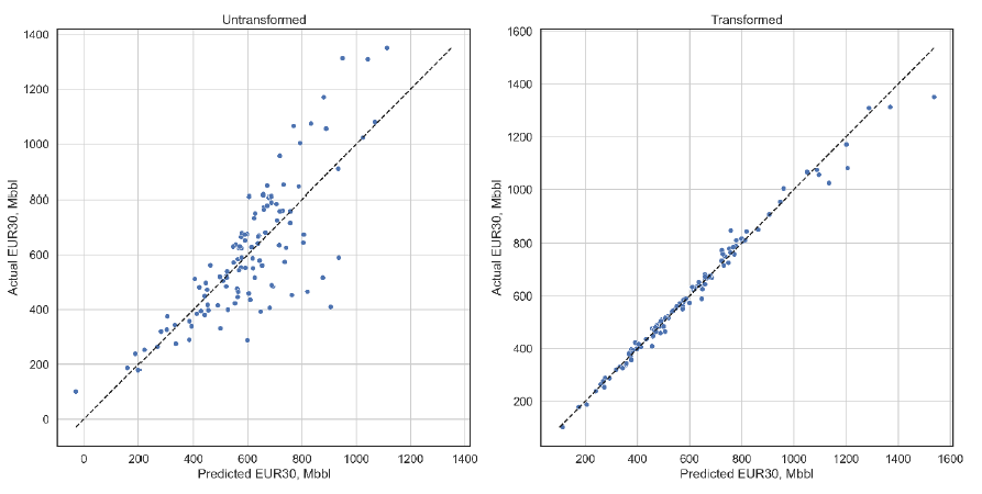
Create a multiple linear regression model to predict log(EUR30) using transformed decline curve parameters, to show how this transformation improve the accuracy of prediction.
Process:
-
Define Predictors and Response:
-
Predictors: Transformed THM parameters (log(qi), log(Di), bi, bf, log(telf)).
-
Response: log(EUR30) from Step 2 forecasts.
-
-
Fit the Model:
-
Use linear regression:
![]()
-
Train on the dataset (e.g., 113 wells in Wolfcamp A) using statistical software (e.g., Python, R).
-
-
Validate the Model:
-
Plot predicted vs. actual log(EUR30).
-
Calculate R2.
-
Check residuals for randomness and homoscedasticity.
-
 = %5cbeta_0 %2b %5cbeta_1 %5ccdot %5clog(q_i) %2b %5cbeta_2 %5ccdot %5clog(D_i) %2b %5cbeta_3 %5ccdot b_i %2b %5cbeta_4 %5ccdot b_f %2b %5cbeta_5 %5ccdot %5clog(t_%7b%5ctext%7belf%7d%7d) %2b %5cepsilon%5cend%7barray%7d%3c/title%3e %3cdefs aria-hidden='true'%3e %3cpath stroke-width='1' id='E1-MJMAIN-6C' d='M42 46H56Q95 46 103 60V68Q103 77 103 91T103 124T104 167T104 217T104 272T104 329Q104 366 104 407T104 482T104 542T103 586T103 603Q100 622 89 628T44 637H26V660Q26 683 28 683L38 684Q48 685 67 686T104 688Q121 689 141 690T171 693T182 694H185V379Q185 62 186 60Q190 52 198 49Q219 46 247 46H263V0H255L232 1Q209 2 183 2T145 3T107 3T57 1L34 0H26V46H42Z'%3e%3c/path%3e %3cpath stroke-width='1' id='E1-MJMAIN-6F' d='M28 214Q28 309 93 378T250 448Q340 448 405 380T471 215Q471 120 407 55T250 -10Q153 -10 91 57T28 214ZM250 30Q372 30 372 193V225V250Q372 272 371 288T364 326T348 362T317 390T268 410Q263 411 252 411Q222 411 195 399Q152 377 139 338T126 246V226Q126 130 145 91Q177 30 250 30Z'%3e%3c/path%3e %3cpath stroke-width='1' id='E1-MJMAIN-67' d='M329 409Q373 453 429 453Q459 453 472 434T485 396Q485 382 476 371T449 360Q416 360 412 390Q410 404 415 411Q415 412 416 414V415Q388 412 363 393Q355 388 355 386Q355 385 359 381T368 369T379 351T388 325T392 292Q392 230 343 187T222 143Q172 143 123 171Q112 153 112 133Q112 98 138 81Q147 75 155 75T227 73Q311 72 335 67Q396 58 431 26Q470 -13 470 -72Q470 -139 392 -175Q332 -206 250 -206Q167 -206 107 -175Q29 -140 29 -75Q29 -39 50 -15T92 18L103 24Q67 55 67 108Q67 155 96 193Q52 237 52 292Q52 355 102 398T223 442Q274 442 318 416L329 409ZM299 343Q294 371 273 387T221 404Q192 404 171 388T145 343Q142 326 142 292Q142 248 149 227T179 192Q196 182 222 182Q244 182 260 189T283 207T294 227T299 242Q302 258 302 292T299 343ZM403 -75Q403 -50 389 -34T348 -11T299 -2T245 0H218Q151 0 138 -6Q118 -15 107 -34T95 -74Q95 -84 101 -97T122 -127T170 -155T250 -167Q319 -167 361 -139T403 -75Z'%3e%3c/path%3e %3cpath stroke-width='1' id='E1-MJMAIN-28' d='M94 250Q94 319 104 381T127 488T164 576T202 643T244 695T277 729T302 750H315H319Q333 750 333 741Q333 738 316 720T275 667T226 581T184 443T167 250T184 58T225 -81T274 -167T316 -220T333 -241Q333 -250 318 -250H315H302L274 -226Q180 -141 137 -14T94 250Z'%3e%3c/path%3e %3cpath stroke-width='1' id='E1-MJMAIN-45' d='M128 619Q121 626 117 628T101 631T58 634H25V680H597V676Q599 670 611 560T625 444V440H585V444Q584 447 582 465Q578 500 570 526T553 571T528 601T498 619T457 629T411 633T353 634Q266 634 251 633T233 622Q233 622 233 621Q232 619 232 497V376H286Q359 378 377 385Q413 401 416 469Q416 471 416 473V493H456V213H416V233Q415 268 408 288T383 317T349 328T297 330Q290 330 286 330H232V196V114Q232 57 237 52Q243 47 289 47H340H391Q428 47 452 50T505 62T552 92T584 146Q594 172 599 200T607 247T612 270V273H652V270Q651 267 632 137T610 3V0H25V46H58Q100 47 109 49T128 61V619Z'%3e%3c/path%3e %3cpath stroke-width='1' id='E1-MJMAIN-55' d='M128 622Q121 629 117 631T101 634T58 637H25V683H36Q57 680 180 680Q315 680 324 683H335V637H302Q262 636 251 634T233 622L232 418V291Q232 189 240 145T280 67Q325 24 389 24Q454 24 506 64T571 183Q575 206 575 410V598Q569 608 565 613T541 627T489 637H472V683H481Q496 680 598 680T715 683H724V637H707Q634 633 622 598L621 399Q620 194 617 180Q617 179 615 171Q595 83 531 31T389 -22Q304 -22 226 33T130 192Q129 201 128 412V622Z'%3e%3c/path%3e %3cpath stroke-width='1' id='E1-MJMAIN-52' d='M130 622Q123 629 119 631T103 634T60 637H27V683H202H236H300Q376 683 417 677T500 648Q595 600 609 517Q610 512 610 501Q610 468 594 439T556 392T511 361T472 343L456 338Q459 335 467 332Q497 316 516 298T545 254T559 211T568 155T578 94Q588 46 602 31T640 16H645Q660 16 674 32T692 87Q692 98 696 101T712 105T728 103T732 90Q732 59 716 27T672 -16Q656 -22 630 -22Q481 -16 458 90Q456 101 456 163T449 246Q430 304 373 320L363 322L297 323H231V192L232 61Q238 51 249 49T301 46H334V0H323Q302 3 181 3Q59 3 38 0H27V46H60Q102 47 111 49T130 61V622ZM491 499V509Q491 527 490 539T481 570T462 601T424 623T362 636Q360 636 340 636T304 637H283Q238 637 234 628Q231 624 231 492V360H289Q390 360 434 378T489 456Q491 467 491 499Z'%3e%3c/path%3e %3cpath stroke-width='1' id='E1-MJMAIN-33' d='M127 463Q100 463 85 480T69 524Q69 579 117 622T233 665Q268 665 277 664Q351 652 390 611T430 522Q430 470 396 421T302 350L299 348Q299 347 308 345T337 336T375 315Q457 262 457 175Q457 96 395 37T238 -22Q158 -22 100 21T42 130Q42 158 60 175T105 193Q133 193 151 175T169 130Q169 119 166 110T159 94T148 82T136 74T126 70T118 67L114 66Q165 21 238 21Q293 21 321 74Q338 107 338 175V195Q338 290 274 322Q259 328 213 329L171 330L168 332Q166 335 166 348Q166 366 174 366Q202 366 232 371Q266 376 294 413T322 525V533Q322 590 287 612Q265 626 240 626Q208 626 181 615T143 592T132 580H135Q138 579 143 578T153 573T165 566T175 555T183 540T186 520Q186 498 172 481T127 463Z'%3e%3c/path%3e %3cpath stroke-width='1' id='E1-MJMAIN-30' d='M96 585Q152 666 249 666Q297 666 345 640T423 548Q460 465 460 320Q460 165 417 83Q397 41 362 16T301 -15T250 -22Q224 -22 198 -16T137 16T82 83Q39 165 39 320Q39 494 96 585ZM321 597Q291 629 250 629Q208 629 178 597Q153 571 145 525T137 333Q137 175 145 125T181 46Q209 16 250 16Q290 16 318 46Q347 76 354 130T362 333Q362 478 354 524T321 597Z'%3e%3c/path%3e %3cpath stroke-width='1' id='E1-MJMAIN-29' d='M60 749L64 750Q69 750 74 750H86L114 726Q208 641 251 514T294 250Q294 182 284 119T261 12T224 -76T186 -143T145 -194T113 -227T90 -246Q87 -249 86 -250H74Q66 -250 63 -250T58 -247T55 -238Q56 -237 66 -225Q221 -64 221 250T66 725Q56 737 55 738Q55 746 60 749Z'%3e%3c/path%3e %3cpath stroke-width='1' id='E1-MJMAIN-3D' d='M56 347Q56 360 70 367H707Q722 359 722 347Q722 336 708 328L390 327H72Q56 332 56 347ZM56 153Q56 168 72 173H708Q722 163 722 153Q722 140 707 133H70Q56 140 56 153Z'%3e%3c/path%3e %3cpath stroke-width='1' id='E1-MJMATHI-3B2' d='M29 -194Q23 -188 23 -186Q23 -183 102 134T186 465Q208 533 243 584T309 658Q365 705 429 705H431Q493 705 533 667T573 570Q573 465 469 396L482 383Q533 332 533 252Q533 139 448 65T257 -10Q227 -10 203 -2T165 17T143 40T131 59T126 65L62 -188Q60 -194 42 -194H29ZM353 431Q392 431 427 419L432 422Q436 426 439 429T449 439T461 453T472 471T484 495T493 524T501 560Q503 569 503 593Q503 611 502 616Q487 667 426 667Q384 667 347 643T286 582T247 514T224 455Q219 439 186 308T152 168Q151 163 151 147Q151 99 173 68Q204 26 260 26Q302 26 349 51T425 137Q441 171 449 214T457 279Q457 337 422 372Q380 358 347 358H337Q258 358 258 389Q258 396 261 403Q275 431 353 431Z'%3e%3c/path%3e %3cpath stroke-width='1' id='E1-MJMAIN-2B' d='M56 237T56 250T70 270H369V420L370 570Q380 583 389 583Q402 583 409 568V270H707Q722 262 722 250T707 230H409V-68Q401 -82 391 -82H389H387Q375 -82 369 -68V230H70Q56 237 56 250Z'%3e%3c/path%3e %3cpath stroke-width='1' id='E1-MJMAIN-31' d='M213 578L200 573Q186 568 160 563T102 556H83V602H102Q149 604 189 617T245 641T273 663Q275 666 285 666Q294 666 302 660V361L303 61Q310 54 315 52T339 48T401 46H427V0H416Q395 3 257 3Q121 3 100 0H88V46H114Q136 46 152 46T177 47T193 50T201 52T207 57T213 61V578Z'%3e%3c/path%3e %3cpath stroke-width='1' id='E1-MJMAIN-22C5' d='M78 250Q78 274 95 292T138 310Q162 310 180 294T199 251Q199 226 182 208T139 190T96 207T78 250Z'%3e%3c/path%3e %3cpath stroke-width='1' id='E1-MJMATHI-71' d='M33 157Q33 258 109 349T280 441Q340 441 372 389Q373 390 377 395T388 406T404 418Q438 442 450 442Q454 442 457 439T460 434Q460 425 391 149Q320 -135 320 -139Q320 -147 365 -148H390Q396 -156 396 -157T393 -175Q389 -188 383 -194H370Q339 -192 262 -192Q234 -192 211 -192T174 -192T157 -193Q143 -193 143 -185Q143 -182 145 -170Q149 -154 152 -151T172 -148Q220 -148 230 -141Q238 -136 258 -53T279 32Q279 33 272 29Q224 -10 172 -10Q117 -10 75 30T33 157ZM352 326Q329 405 277 405Q242 405 210 374T160 293Q131 214 119 129Q119 126 119 118T118 106Q118 61 136 44T179 26Q233 26 290 98L298 109L352 326Z'%3e%3c/path%3e %3cpath stroke-width='1' id='E1-MJMATHI-69' d='M184 600Q184 624 203 642T247 661Q265 661 277 649T290 619Q290 596 270 577T226 557Q211 557 198 567T184 600ZM21 287Q21 295 30 318T54 369T98 420T158 442Q197 442 223 419T250 357Q250 340 236 301T196 196T154 83Q149 61 149 51Q149 26 166 26Q175 26 185 29T208 43T235 78T260 137Q263 149 265 151T282 153Q302 153 302 143Q302 135 293 112T268 61T223 11T161 -11Q129 -11 102 10T74 74Q74 91 79 106T122 220Q160 321 166 341T173 380Q173 404 156 404H154Q124 404 99 371T61 287Q60 286 59 284T58 281T56 279T53 278T49 278T41 278H27Q21 284 21 287Z'%3e%3c/path%3e %3cpath stroke-width='1' id='E1-MJMAIN-32' d='M109 429Q82 429 66 447T50 491Q50 562 103 614T235 666Q326 666 387 610T449 465Q449 422 429 383T381 315T301 241Q265 210 201 149L142 93L218 92Q375 92 385 97Q392 99 409 186V189H449V186Q448 183 436 95T421 3V0H50V19V31Q50 38 56 46T86 81Q115 113 136 137Q145 147 170 174T204 211T233 244T261 278T284 308T305 340T320 369T333 401T340 431T343 464Q343 527 309 573T212 619Q179 619 154 602T119 569T109 550Q109 549 114 549Q132 549 151 535T170 489Q170 464 154 447T109 429Z'%3e%3c/path%3e %3cpath stroke-width='1' id='E1-MJMATHI-44' d='M287 628Q287 635 230 637Q207 637 200 638T193 647Q193 655 197 667T204 682Q206 683 403 683Q570 682 590 682T630 676Q702 659 752 597T803 431Q803 275 696 151T444 3L430 1L236 0H125H72Q48 0 41 2T33 11Q33 13 36 25Q40 41 44 43T67 46Q94 46 127 49Q141 52 146 61Q149 65 218 339T287 628ZM703 469Q703 507 692 537T666 584T629 613T590 629T555 636Q553 636 541 636T512 636T479 637H436Q392 637 386 627Q384 623 313 339T242 52Q242 48 253 48T330 47Q335 47 349 47T373 46Q499 46 581 128Q617 164 640 212T683 339T703 469Z'%3e%3c/path%3e %3cpath stroke-width='1' id='E1-MJMATHI-62' d='M73 647Q73 657 77 670T89 683Q90 683 161 688T234 694Q246 694 246 685T212 542Q204 508 195 472T180 418L176 399Q176 396 182 402Q231 442 283 442Q345 442 383 396T422 280Q422 169 343 79T173 -11Q123 -11 82 27T40 150V159Q40 180 48 217T97 414Q147 611 147 623T109 637Q104 637 101 637H96Q86 637 83 637T76 640T73 647ZM336 325V331Q336 405 275 405Q258 405 240 397T207 376T181 352T163 330L157 322L136 236Q114 150 114 114Q114 66 138 42Q154 26 178 26Q211 26 245 58Q270 81 285 114T318 219Q336 291 336 325Z'%3e%3c/path%3e %3cpath stroke-width='1' id='E1-MJMAIN-34' d='M462 0Q444 3 333 3Q217 3 199 0H190V46H221Q241 46 248 46T265 48T279 53T286 61Q287 63 287 115V165H28V211L179 442Q332 674 334 675Q336 677 355 677H373L379 671V211H471V165H379V114Q379 73 379 66T385 54Q393 47 442 46H471V0H462ZM293 211V545L74 212L183 211H293Z'%3e%3c/path%3e %3cpath stroke-width='1' id='E1-MJMATHI-66' d='M118 -162Q120 -162 124 -164T135 -167T147 -168Q160 -168 171 -155T187 -126Q197 -99 221 27T267 267T289 382V385H242Q195 385 192 387Q188 390 188 397L195 425Q197 430 203 430T250 431Q298 431 298 432Q298 434 307 482T319 540Q356 705 465 705Q502 703 526 683T550 630Q550 594 529 578T487 561Q443 561 443 603Q443 622 454 636T478 657L487 662Q471 668 457 668Q445 668 434 658T419 630Q412 601 403 552T387 469T380 433Q380 431 435 431Q480 431 487 430T498 424Q499 420 496 407T491 391Q489 386 482 386T428 385H372L349 263Q301 15 282 -47Q255 -132 212 -173Q175 -205 139 -205Q107 -205 81 -186T55 -132Q55 -95 76 -78T118 -61Q162 -61 162 -103Q162 -122 151 -136T127 -157L118 -162Z'%3e%3c/path%3e %3cpath stroke-width='1' id='E1-MJMAIN-35' d='M164 157Q164 133 148 117T109 101H102Q148 22 224 22Q294 22 326 82Q345 115 345 210Q345 313 318 349Q292 382 260 382H254Q176 382 136 314Q132 307 129 306T114 304Q97 304 95 310Q93 314 93 485V614Q93 664 98 664Q100 666 102 666Q103 666 123 658T178 642T253 634Q324 634 389 662Q397 666 402 666Q410 666 410 648V635Q328 538 205 538Q174 538 149 544L139 546V374Q158 388 169 396T205 412T256 420Q337 420 393 355T449 201Q449 109 385 44T229 -22Q148 -22 99 32T50 154Q50 178 61 192T84 210T107 214Q132 214 148 197T164 157Z'%3e%3c/path%3e %3cpath stroke-width='1' id='E1-MJMATHI-74' d='M26 385Q19 392 19 395Q19 399 22 411T27 425Q29 430 36 430T87 431H140L159 511Q162 522 166 540T173 566T179 586T187 603T197 615T211 624T229 626Q247 625 254 615T261 596Q261 589 252 549T232 470L222 433Q222 431 272 431H323Q330 424 330 420Q330 398 317 385H210L174 240Q135 80 135 68Q135 26 162 26Q197 26 230 60T283 144Q285 150 288 151T303 153H307Q322 153 322 145Q322 142 319 133Q314 117 301 95T267 48T216 6T155 -11Q125 -11 98 4T59 56Q57 64 57 83V101L92 241Q127 382 128 383Q128 385 77 385H26Z'%3e%3c/path%3e %3cpath stroke-width='1' id='E1-MJMAIN-65' d='M28 218Q28 273 48 318T98 391T163 433T229 448Q282 448 320 430T378 380T406 316T415 245Q415 238 408 231H126V216Q126 68 226 36Q246 30 270 30Q312 30 342 62Q359 79 369 104L379 128Q382 131 395 131H398Q415 131 415 121Q415 117 412 108Q393 53 349 21T250 -11Q155 -11 92 58T28 218ZM333 275Q322 403 238 411H236Q228 411 220 410T195 402T166 381T143 340T127 274V267H333V275Z'%3e%3c/path%3e %3cpath stroke-width='1' id='E1-MJMAIN-66' d='M273 0Q255 3 146 3Q43 3 34 0H26V46H42Q70 46 91 49Q99 52 103 60Q104 62 104 224V385H33V431H104V497L105 564L107 574Q126 639 171 668T266 704Q267 704 275 704T289 705Q330 702 351 679T372 627Q372 604 358 590T321 576T284 590T270 627Q270 647 288 667H284Q280 668 273 668Q245 668 223 647T189 592Q183 572 182 497V431H293V385H185V225Q185 63 186 61T189 57T194 54T199 51T206 49T213 48T222 47T231 47T241 46T251 46H282V0H273Z'%3e%3c/path%3e %3cpath stroke-width='1' id='E1-MJMATHI-3F5' d='M227 -11Q149 -11 95 41T40 174Q40 262 87 322Q121 367 173 396T287 430Q289 431 329 431H367Q382 426 382 411Q382 385 341 385H325H312Q191 385 154 277L150 265H327Q340 256 340 246Q340 228 320 219H138V217Q128 187 128 143Q128 77 160 52T231 26Q258 26 284 36T326 57T343 68Q350 68 354 58T358 39Q358 36 357 35Q354 31 337 21T289 0T227 -11Z'%3e%3c/path%3e %3c/defs%3e %3cg stroke='currentColor' fill='currentColor' stroke-width='0' transform='matrix(1 0 0 -1 0 0)' aria-hidden='true'%3e %3cg transform='translate(167%2c0)'%3e %3cg transform='translate(-11%2c0)'%3e %3cuse xlink:href='%23E1-MJMAIN-6C'%3e%3c/use%3e %3cuse xlink:href='%23E1-MJMAIN-6F' x='278' y='0'%3e%3c/use%3e %3cuse xlink:href='%23E1-MJMAIN-67' x='779' y='0'%3e%3c/use%3e %3cuse xlink:href='%23E1-MJMAIN-28' x='1279' y='0'%3e%3c/use%3e %3cg transform='translate(1669%2c0)'%3e %3cuse xlink:href='%23E1-MJMAIN-45'%3e%3c/use%3e %3cuse xlink:href='%23E1-MJMAIN-55' x='681' y='0'%3e%3c/use%3e %3cuse xlink:href='%23E1-MJMAIN-52' x='1432' y='0'%3e%3c/use%3e %3cg transform='translate(2168%2c-150)'%3e %3cuse transform='scale(0.707)' xlink:href='%23E1-MJMAIN-33'%3e%3c/use%3e %3cuse transform='scale(0.707)' xlink:href='%23E1-MJMAIN-30' x='500' y='0'%3e%3c/use%3e %3c/g%3e %3c/g%3e %3cuse xlink:href='%23E1-MJMAIN-29' x='4645' y='0'%3e%3c/use%3e %3cuse xlink:href='%23E1-MJMAIN-3D' x='5312' y='0'%3e%3c/use%3e %3cg transform='translate(6368%2c0)'%3e %3cuse xlink:href='%23E1-MJMATHI-3B2' x='0' y='0'%3e%3c/use%3e %3cuse transform='scale(0.707)' xlink:href='%23E1-MJMAIN-30' x='801' y='-213'%3e%3c/use%3e %3c/g%3e %3cuse xlink:href='%23E1-MJMAIN-2B' x='7611' y='0'%3e%3c/use%3e %3cg transform='translate(8612%2c0)'%3e %3cuse xlink:href='%23E1-MJMATHI-3B2' x='0' y='0'%3e%3c/use%3e %3cuse transform='scale(0.707)' xlink:href='%23E1-MJMAIN-31' x='801' y='-213'%3e%3c/use%3e %3c/g%3e %3cuse xlink:href='%23E1-MJMAIN-22C5' x='9854' y='0'%3e%3c/use%3e %3cg transform='translate(10355%2c0)'%3e %3cuse xlink:href='%23E1-MJMAIN-6C'%3e%3c/use%3e %3cuse xlink:href='%23E1-MJMAIN-6F' x='278' y='0'%3e%3c/use%3e %3cuse xlink:href='%23E1-MJMAIN-67' x='779' y='0'%3e%3c/use%3e %3c/g%3e %3cuse xlink:href='%23E1-MJMAIN-28' x='11635' y='0'%3e%3c/use%3e %3cg transform='translate(12024%2c0)'%3e %3cuse xlink:href='%23E1-MJMATHI-71' x='0' y='0'%3e%3c/use%3e %3cuse transform='scale(0.707)' xlink:href='%23E1-MJMATHI-69' x='631' y='-213'%3e%3c/use%3e %3c/g%3e %3cuse xlink:href='%23E1-MJMAIN-29' x='12815' y='0'%3e%3c/use%3e %3cuse xlink:href='%23E1-MJMAIN-2B' x='13427' y='0'%3e%3c/use%3e %3cg transform='translate(14427%2c0)'%3e %3cuse xlink:href='%23E1-MJMATHI-3B2' x='0' y='0'%3e%3c/use%3e %3cuse transform='scale(0.707)' xlink:href='%23E1-MJMAIN-32' x='801' y='-213'%3e%3c/use%3e %3c/g%3e %3cuse xlink:href='%23E1-MJMAIN-22C5' x='15670' y='0'%3e%3c/use%3e %3cg transform='translate(16171%2c0)'%3e %3cuse xlink:href='%23E1-MJMAIN-6C'%3e%3c/use%3e %3cuse xlink:href='%23E1-MJMAIN-6F' x='278' y='0'%3e%3c/use%3e %3cuse xlink:href='%23E1-MJMAIN-67' x='779' y='0'%3e%3c/use%3e %3c/g%3e %3cuse xlink:href='%23E1-MJMAIN-28' x='17450' y='0'%3e%3c/use%3e %3cg transform='translate(17840%2c0)'%3e %3cuse xlink:href='%23E1-MJMATHI-44' x='0' y='0'%3e%3c/use%3e %3cuse transform='scale(0.707)' xlink:href='%23E1-MJMATHI-69' x='1171' y='-213'%3e%3c/use%3e %3c/g%3e %3cuse xlink:href='%23E1-MJMAIN-29' x='19012' y='0'%3e%3c/use%3e %3cuse xlink:href='%23E1-MJMAIN-2B' x='19624' y='0'%3e%3c/use%3e %3cg transform='translate(20625%2c0)'%3e %3cuse xlink:href='%23E1-MJMATHI-3B2' x='0' y='0'%3e%3c/use%3e %3cuse transform='scale(0.707)' xlink:href='%23E1-MJMAIN-33' x='801' y='-213'%3e%3c/use%3e %3c/g%3e %3cuse xlink:href='%23E1-MJMAIN-22C5' x='21868' y='0'%3e%3c/use%3e %3cg transform='translate(22368%2c0)'%3e %3cuse xlink:href='%23E1-MJMATHI-62' x='0' y='0'%3e%3c/use%3e %3cuse transform='scale(0.707)' xlink:href='%23E1-MJMATHI-69' x='607' y='-213'%3e%3c/use%3e %3c/g%3e %3cuse xlink:href='%23E1-MJMAIN-2B' x='23364' y='0'%3e%3c/use%3e %3cg transform='translate(24365%2c0)'%3e %3cuse xlink:href='%23E1-MJMATHI-3B2' x='0' y='0'%3e%3c/use%3e %3cuse transform='scale(0.707)' xlink:href='%23E1-MJMAIN-34' x='801' y='-213'%3e%3c/use%3e %3c/g%3e %3cuse xlink:href='%23E1-MJMAIN-22C5' x='25608' y='0'%3e%3c/use%3e %3cg transform='translate(26108%2c0)'%3e %3cuse xlink:href='%23E1-MJMATHI-62' x='0' y='0'%3e%3c/use%3e %3cuse transform='scale(0.707)' xlink:href='%23E1-MJMATHI-66' x='607' y='-219'%3e%3c/use%3e %3c/g%3e %3cuse xlink:href='%23E1-MJMAIN-2B' x='27249' y='0'%3e%3c/use%3e %3cg transform='translate(28250%2c0)'%3e %3cuse xlink:href='%23E1-MJMATHI-3B2' x='0' y='0'%3e%3c/use%3e %3cuse transform='scale(0.707)' xlink:href='%23E1-MJMAIN-35' x='801' y='-213'%3e%3c/use%3e %3c/g%3e %3cuse xlink:href='%23E1-MJMAIN-22C5' x='29493' y='0'%3e%3c/use%3e %3cg transform='translate(29993%2c0)'%3e %3cuse xlink:href='%23E1-MJMAIN-6C'%3e%3c/use%3e %3cuse xlink:href='%23E1-MJMAIN-6F' x='278' y='0'%3e%3c/use%3e %3cuse xlink:href='%23E1-MJMAIN-67' x='779' y='0'%3e%3c/use%3e %3c/g%3e %3cuse xlink:href='%23E1-MJMAIN-28' x='31273' y='0'%3e%3c/use%3e %3cg transform='translate(31662%2c0)'%3e %3cuse xlink:href='%23E1-MJMATHI-74' x='0' y='0'%3e%3c/use%3e %3cg transform='translate(361%2c-155)'%3e %3cuse transform='scale(0.707)' xlink:href='%23E1-MJMAIN-65'%3e%3c/use%3e %3cuse transform='scale(0.707)' xlink:href='%23E1-MJMAIN-6C' x='444' y='0'%3e%3c/use%3e %3cuse transform='scale(0.707)' xlink:href='%23E1-MJMAIN-66' x='723' y='0'%3e%3c/use%3e %3c/g%3e %3c/g%3e %3cuse xlink:href='%23E1-MJMAIN-29' x='32852' y='0'%3e%3c/use%3e %3cuse xlink:href='%23E1-MJMAIN-2B' x='33464' y='0'%3e%3c/use%3e %3cuse xlink:href='%23E1-MJMATHI-3F5' x='34464' y='0'%3e%3c/use%3e %3c/g%3e %3c/g%3e %3c/g%3e %3c/svg%3e)
Considerations:
-
Transformations normalize distributions, ensuring model validity.
-
High R2 indicates robustness, but TWP time-rate behavior (Step 6) is the ultimate test.
-
Use consistent forecasting (Step 2) to avoid errors.
Step 5: Compute the TWP Parameters
Derive the TWP by calculating the arithmetic mean of the transformed parameters and reversing the transformations.
-
Process:
-
Compute the arithmetic mean of each transformed parameter across all wells:
-
Mean of log(qi)
-
Mean of log(Di)
-
Mean of bi
-
Mean of bf
-
Mean of log(telf)
-
-
Reverse the transformations to obtain the TWP parameters (Using the following formula):
![]()
-
qi: exp (mean of log(qi))
-
Di : exp (mean of log(Di))
-
bi: No transformation (use mean of bi)
-
bf: No transformation (use mean of bf)
-
telf : exp (mean of log(telf))
-
-
Use these parameters in the THM rate function (below equation) to generate the TWP time-rate profile (Fulford and Blasingame 2013).
![]()
-
-
Considerations:
-
The resulting TWP EUR is typically close to the P50 of the well set’s EUR distribution (Figure 4).
-
If the TWP EUR deviates significantly from the P50, apply a scalar correction to the initial rate (qi) to calibrate it.
-
%5e%7b-1%7d = %5cbegin%7bcases%7d y%5e%7b1 / %5clambda%7d %26amp%3b %5clambda %5cneq 0 %5c%5c %5cexp y %26amp%3b %5clambda = 0 %5cend%7bcases%7d %5cend%7baligned%7d%3c/title%3e %3cdefs aria-hidden='true'%3e %3cpath stroke-width='1' id='E1-MJMATHI-66' d='M118 -162Q120 -162 124 -164T135 -167T147 -168Q160 -168 171 -155T187 -126Q197 -99 221 27T267 267T289 382V385H242Q195 385 192 387Q188 390 188 397L195 425Q197 430 203 430T250 431Q298 431 298 432Q298 434 307 482T319 540Q356 705 465 705Q502 703 526 683T550 630Q550 594 529 578T487 561Q443 561 443 603Q443 622 454 636T478 657L487 662Q471 668 457 668Q445 668 434 658T419 630Q412 601 403 552T387 469T380 433Q380 431 435 431Q480 431 487 430T498 424Q499 420 496 407T491 391Q489 386 482 386T428 385H372L349 263Q301 15 282 -47Q255 -132 212 -173Q175 -205 139 -205Q107 -205 81 -186T55 -132Q55 -95 76 -78T118 -61Q162 -61 162 -103Q162 -122 151 -136T127 -157L118 -162Z'%3e%3c/path%3e %3cpath stroke-width='1' id='E1-MJMAIN-28' d='M94 250Q94 319 104 381T127 488T164 576T202 643T244 695T277 729T302 750H315H319Q333 750 333 741Q333 738 316 720T275 667T226 581T184 443T167 250T184 58T225 -81T274 -167T316 -220T333 -241Q333 -250 318 -250H315H302L274 -226Q180 -141 137 -14T94 250Z'%3e%3c/path%3e %3cpath stroke-width='1' id='E1-MJMATHI-79' d='M21 287Q21 301 36 335T84 406T158 442Q199 442 224 419T250 355Q248 336 247 334Q247 331 231 288T198 191T182 105Q182 62 196 45T238 27Q261 27 281 38T312 61T339 94Q339 95 344 114T358 173T377 247Q415 397 419 404Q432 431 462 431Q475 431 483 424T494 412T496 403Q496 390 447 193T391 -23Q363 -106 294 -155T156 -205Q111 -205 77 -183T43 -117Q43 -95 50 -80T69 -58T89 -48T106 -45Q150 -45 150 -87Q150 -107 138 -122T115 -142T102 -147L99 -148Q101 -153 118 -160T152 -167H160Q177 -167 186 -165Q219 -156 247 -127T290 -65T313 -9T321 21L315 17Q309 13 296 6T270 -6Q250 -11 231 -11Q185 -11 150 11T104 82Q103 89 103 113Q103 170 138 262T173 379Q173 380 173 381Q173 390 173 393T169 400T158 404H154Q131 404 112 385T82 344T65 302T57 280Q55 278 41 278H27Q21 284 21 287Z'%3e%3c/path%3e %3cpath stroke-width='1' id='E1-MJMAIN-2C' d='M78 35T78 60T94 103T137 121Q165 121 187 96T210 8Q210 -27 201 -60T180 -117T154 -158T130 -185T117 -194Q113 -194 104 -185T95 -172Q95 -168 106 -156T131 -126T157 -76T173 -3V9L172 8Q170 7 167 6T161 3T152 1T140 0Q113 0 96 17Z'%3e%3c/path%3e %3cpath stroke-width='1' id='E1-MJMATHI-3BB' d='M166 673Q166 685 183 694H202Q292 691 316 644Q322 629 373 486T474 207T524 67Q531 47 537 34T546 15T551 6T555 2T556 -2T550 -11H482Q457 3 450 18T399 152L354 277L340 262Q327 246 293 207T236 141Q211 112 174 69Q123 9 111 -1T83 -12Q47 -12 47 20Q47 37 61 52T199 187Q229 216 266 252T321 306L338 322Q338 323 288 462T234 612Q214 657 183 657Q166 657 166 673Z'%3e%3c/path%3e %3cpath stroke-width='1' id='E1-MJMAIN-29' d='M60 749L64 750Q69 750 74 750H86L114 726Q208 641 251 514T294 250Q294 182 284 119T261 12T224 -76T186 -143T145 -194T113 -227T90 -246Q87 -249 86 -250H74Q66 -250 63 -250T58 -247T55 -238Q56 -237 66 -225Q221 -64 221 250T66 725Q56 737 55 738Q55 746 60 749Z'%3e%3c/path%3e %3cpath stroke-width='1' id='E1-MJMAIN-2212' d='M84 237T84 250T98 270H679Q694 262 694 250T679 230H98Q84 237 84 250Z'%3e%3c/path%3e %3cpath stroke-width='1' id='E1-MJMAIN-31' d='M213 578L200 573Q186 568 160 563T102 556H83V602H102Q149 604 189 617T245 641T273 663Q275 666 285 666Q294 666 302 660V361L303 61Q310 54 315 52T339 48T401 46H427V0H416Q395 3 257 3Q121 3 100 0H88V46H114Q136 46 152 46T177 47T193 50T201 52T207 57T213 61V578Z'%3e%3c/path%3e %3cpath stroke-width='1' id='E1-MJMAIN-3D' d='M56 347Q56 360 70 367H707Q722 359 722 347Q722 336 708 328L390 327H72Q56 332 56 347ZM56 153Q56 168 72 173H708Q722 163 722 153Q722 140 707 133H70Q56 140 56 153Z'%3e%3c/path%3e %3cpath stroke-width='1' id='E1-MJMAIN-7B' d='M434 -231Q434 -244 428 -250H410Q281 -250 230 -184Q225 -177 222 -172T217 -161T213 -148T211 -133T210 -111T209 -84T209 -47T209 0Q209 21 209 53Q208 142 204 153Q203 154 203 155Q189 191 153 211T82 231Q71 231 68 234T65 250T68 266T82 269Q116 269 152 289T203 345Q208 356 208 377T209 529V579Q209 634 215 656T244 698Q270 724 324 740Q361 748 377 749Q379 749 390 749T408 750H428Q434 744 434 732Q434 719 431 716Q429 713 415 713Q362 710 332 689T296 647Q291 634 291 499V417Q291 370 288 353T271 314Q240 271 184 255L170 250L184 245Q202 239 220 230T262 196T290 137Q291 131 291 1Q291 -134 296 -147Q306 -174 339 -192T415 -213Q429 -213 431 -216Q434 -219 434 -231Z'%3e%3c/path%3e %3cpath stroke-width='1' id='E1-MJMAIN-2F' d='M423 750Q432 750 438 744T444 730Q444 725 271 248T92 -240Q85 -250 75 -250Q68 -250 62 -245T56 -231Q56 -221 230 257T407 740Q411 750 423 750Z'%3e%3c/path%3e %3cpath stroke-width='1' id='E1-MJMAIN-2260' d='M166 -215T159 -215T147 -212T141 -204T139 -197Q139 -190 144 -183L306 133H70Q56 140 56 153Q56 168 72 173H327L406 327H72Q56 332 56 347Q56 360 70 367H426Q597 702 602 707Q605 716 618 716Q625 716 630 712T636 703T638 696Q638 692 471 367H707Q722 359 722 347Q722 336 708 328L451 327L371 173H708Q722 163 722 153Q722 140 707 133H351Q175 -210 170 -212Q166 -215 159 -215Z'%3e%3c/path%3e %3cpath stroke-width='1' id='E1-MJMAIN-30' d='M96 585Q152 666 249 666Q297 666 345 640T423 548Q460 465 460 320Q460 165 417 83Q397 41 362 16T301 -15T250 -22Q224 -22 198 -16T137 16T82 83Q39 165 39 320Q39 494 96 585ZM321 597Q291 629 250 629Q208 629 178 597Q153 571 145 525T137 333Q137 175 145 125T181 46Q209 16 250 16Q290 16 318 46Q347 76 354 130T362 333Q362 478 354 524T321 597Z'%3e%3c/path%3e %3cpath stroke-width='1' id='E1-MJMAIN-65' d='M28 218Q28 273 48 318T98 391T163 433T229 448Q282 448 320 430T378 380T406 316T415 245Q415 238 408 231H126V216Q126 68 226 36Q246 30 270 30Q312 30 342 62Q359 79 369 104L379 128Q382 131 395 131H398Q415 131 415 121Q415 117 412 108Q393 53 349 21T250 -11Q155 -11 92 58T28 218ZM333 275Q322 403 238 411H236Q228 411 220 410T195 402T166 381T143 340T127 274V267H333V275Z'%3e%3c/path%3e %3cpath stroke-width='1' id='E1-MJMAIN-78' d='M201 0Q189 3 102 3Q26 3 17 0H11V46H25Q48 47 67 52T96 61T121 78T139 96T160 122T180 150L226 210L168 288Q159 301 149 315T133 336T122 351T113 363T107 370T100 376T94 379T88 381T80 383Q74 383 44 385H16V431H23Q59 429 126 429Q219 429 229 431H237V385Q201 381 201 369Q201 367 211 353T239 315T268 274L272 270L297 304Q329 345 329 358Q329 364 327 369T322 376T317 380T310 384L307 385H302V431H309Q324 428 408 428Q487 428 493 431H499V385H492Q443 385 411 368Q394 360 377 341T312 257L296 236L358 151Q424 61 429 57T446 50Q464 46 499 46H516V0H510H502Q494 1 482 1T457 2T432 2T414 3Q403 3 377 3T327 1L304 0H295V46H298Q309 46 320 51T331 63Q331 65 291 120L250 175Q249 174 219 133T185 88Q181 83 181 74Q181 63 188 55T206 46Q208 46 208 23V0H201Z'%3e%3c/path%3e %3cpath stroke-width='1' id='E1-MJMAIN-70' d='M36 -148H50Q89 -148 97 -134V-126Q97 -119 97 -107T97 -77T98 -38T98 6T98 55T98 106Q98 140 98 177T98 243T98 296T97 335T97 351Q94 370 83 376T38 385H20V408Q20 431 22 431L32 432Q42 433 61 434T98 436Q115 437 135 438T165 441T176 442H179V416L180 390L188 397Q247 441 326 441Q407 441 464 377T522 216Q522 115 457 52T310 -11Q242 -11 190 33L182 40V-45V-101Q182 -128 184 -134T195 -145Q216 -148 244 -148H260V-194H252L228 -193Q205 -192 178 -192T140 -191Q37 -191 28 -194H20V-148H36ZM424 218Q424 292 390 347T305 402Q234 402 182 337V98Q222 26 294 26Q345 26 384 80T424 218Z'%3e%3c/path%3e %3cpath stroke-width='1' id='E1-MJSZ3-7B' d='M618 -943L612 -949H582L568 -943Q472 -903 411 -841T332 -703Q327 -682 327 -653T325 -350Q324 -28 323 -18Q317 24 301 61T264 124T221 171T179 205T147 225T132 234Q130 238 130 250Q130 255 130 258T131 264T132 267T134 269T139 272T144 275Q207 308 256 367Q310 436 323 519Q324 529 325 851Q326 1124 326 1154T332 1205Q369 1358 566 1443L582 1450H612L618 1444V1429Q618 1413 616 1411L608 1406Q599 1402 585 1393T552 1372T515 1343T479 1305T449 1257T429 1200Q425 1180 425 1152T423 851Q422 579 422 549T416 498Q407 459 388 424T346 364T297 318T250 284T214 264T197 254L188 251L205 242Q290 200 345 138T416 3Q421 -18 421 -48T423 -349Q423 -397 423 -472Q424 -677 428 -694Q429 -697 429 -699Q434 -722 443 -743T465 -782T491 -816T519 -845T548 -868T574 -886T595 -899T610 -908L616 -910Q618 -912 618 -928V-943Z'%3e%3c/path%3e %3c/defs%3e %3cg stroke='currentColor' fill='currentColor' stroke-width='0' transform='matrix(1 0 0 -1 0 0)' aria-hidden='true'%3e %3cg transform='translate(167%2c0)'%3e %3cg transform='translate(-11%2c0)'%3e %3cuse xlink:href='%23E1-MJMATHI-66' x='0' y='0'%3e%3c/use%3e %3cuse xlink:href='%23E1-MJMAIN-28' x='550' y='0'%3e%3c/use%3e %3cuse xlink:href='%23E1-MJMATHI-79' x='940' y='0'%3e%3c/use%3e %3cuse xlink:href='%23E1-MJMAIN-2C' x='1437' y='0'%3e%3c/use%3e %3cuse xlink:href='%23E1-MJMATHI-3BB' x='1882' y='0'%3e%3c/use%3e %3cg transform='translate(2466%2c0)'%3e %3cuse xlink:href='%23E1-MJMAIN-29' x='0' y='0'%3e%3c/use%3e %3cg transform='translate(389%2c412)'%3e %3cuse transform='scale(0.707)' xlink:href='%23E1-MJMAIN-2212' x='0' y='0'%3e%3c/use%3e %3cuse transform='scale(0.707)' xlink:href='%23E1-MJMAIN-31' x='778' y='0'%3e%3c/use%3e %3c/g%3e %3c/g%3e %3cuse xlink:href='%23E1-MJMAIN-3D' x='4137' y='0'%3e%3c/use%3e %3cg transform='translate(5194%2c0)'%3e %3cuse xlink:href='%23E1-MJSZ3-7B'%3e%3c/use%3e %3cg transform='translate(917%2c0)'%3e %3cg transform='translate(-11%2c0)'%3e %3cg transform='translate(0%2c514)'%3e %3cuse xlink:href='%23E1-MJMATHI-79' x='0' y='0'%3e%3c/use%3e %3cg transform='translate(499%2c362)'%3e %3cuse transform='scale(0.707)' xlink:href='%23E1-MJMAIN-31' x='0' y='0'%3e%3c/use%3e %3cuse transform='scale(0.707)' xlink:href='%23E1-MJMAIN-2F' x='500' y='0'%3e%3c/use%3e %3cuse transform='scale(0.707)' xlink:href='%23E1-MJMATHI-3BB' x='1001' y='0'%3e%3c/use%3e %3c/g%3e %3c/g%3e %3cg transform='translate(0%2c-702)'%3e %3cuse xlink:href='%23E1-MJMAIN-65'%3e%3c/use%3e %3cuse xlink:href='%23E1-MJMAIN-78' x='444' y='0'%3e%3c/use%3e %3cuse xlink:href='%23E1-MJMAIN-70' x='973' y='0'%3e%3c/use%3e %3cuse xlink:href='%23E1-MJMATHI-79' x='1696' y='0'%3e%3c/use%3e %3c/g%3e %3c/g%3e %3cg transform='translate(3183%2c0)'%3e %3cg transform='translate(0%2c514)'%3e %3cuse xlink:href='%23E1-MJMATHI-3BB' x='0' y='0'%3e%3c/use%3e %3cuse xlink:href='%23E1-MJMAIN-2260' x='861' y='0'%3e%3c/use%3e %3cuse xlink:href='%23E1-MJMAIN-30' x='1917' y='0'%3e%3c/use%3e %3c/g%3e %3cg transform='translate(0%2c-702)'%3e %3cuse xlink:href='%23E1-MJMATHI-3BB' x='0' y='0'%3e%3c/use%3e %3cuse xlink:href='%23E1-MJMAIN-3D' x='861' y='0'%3e%3c/use%3e %3cuse xlink:href='%23E1-MJMAIN-30' x='1917' y='0'%3e%3c/use%3e %3c/g%3e %3c/g%3e %3c/g%3e %3c/g%3e %3c/g%3e %3c/g%3e %3c/g%3e %3c/svg%3e)
 = f%5cleft(q_i%2c D_i%2c b_i%2c b_f%2c t_%7belf%7d%5cright)%5cend%7barray%7d%3c/title%3e %3cdefs aria-hidden='true'%3e %3cpath stroke-width='1' id='E1-MJMATHI-71' d='M33 157Q33 258 109 349T280 441Q340 441 372 389Q373 390 377 395T388 406T404 418Q438 442 450 442Q454 442 457 439T460 434Q460 425 391 149Q320 -135 320 -139Q320 -147 365 -148H390Q396 -156 396 -157T393 -175Q389 -188 383 -194H370Q339 -192 262 -192Q234 -192 211 -192T174 -192T157 -193Q143 -193 143 -185Q143 -182 145 -170Q149 -154 152 -151T172 -148Q220 -148 230 -141Q238 -136 258 -53T279 32Q279 33 272 29Q224 -10 172 -10Q117 -10 75 30T33 157ZM352 326Q329 405 277 405Q242 405 210 374T160 293Q131 214 119 129Q119 126 119 118T118 106Q118 61 136 44T179 26Q233 26 290 98L298 109L352 326Z'%3e%3c/path%3e %3cpath stroke-width='1' id='E1-MJMAIN-28' d='M94 250Q94 319 104 381T127 488T164 576T202 643T244 695T277 729T302 750H315H319Q333 750 333 741Q333 738 316 720T275 667T226 581T184 443T167 250T184 58T225 -81T274 -167T316 -220T333 -241Q333 -250 318 -250H315H302L274 -226Q180 -141 137 -14T94 250Z'%3e%3c/path%3e %3cpath stroke-width='1' id='E1-MJMATHI-74' d='M26 385Q19 392 19 395Q19 399 22 411T27 425Q29 430 36 430T87 431H140L159 511Q162 522 166 540T173 566T179 586T187 603T197 615T211 624T229 626Q247 625 254 615T261 596Q261 589 252 549T232 470L222 433Q222 431 272 431H323Q330 424 330 420Q330 398 317 385H210L174 240Q135 80 135 68Q135 26 162 26Q197 26 230 60T283 144Q285 150 288 151T303 153H307Q322 153 322 145Q322 142 319 133Q314 117 301 95T267 48T216 6T155 -11Q125 -11 98 4T59 56Q57 64 57 83V101L92 241Q127 382 128 383Q128 385 77 385H26Z'%3e%3c/path%3e %3cpath stroke-width='1' id='E1-MJMAIN-29' d='M60 749L64 750Q69 750 74 750H86L114 726Q208 641 251 514T294 250Q294 182 284 119T261 12T224 -76T186 -143T145 -194T113 -227T90 -246Q87 -249 86 -250H74Q66 -250 63 -250T58 -247T55 -238Q56 -237 66 -225Q221 -64 221 250T66 725Q56 737 55 738Q55 746 60 749Z'%3e%3c/path%3e %3cpath stroke-width='1' id='E1-MJMAIN-3D' d='M56 347Q56 360 70 367H707Q722 359 722 347Q722 336 708 328L390 327H72Q56 332 56 347ZM56 153Q56 168 72 173H708Q722 163 722 153Q722 140 707 133H70Q56 140 56 153Z'%3e%3c/path%3e %3cpath stroke-width='1' id='E1-MJMATHI-66' d='M118 -162Q120 -162 124 -164T135 -167T147 -168Q160 -168 171 -155T187 -126Q197 -99 221 27T267 267T289 382V385H242Q195 385 192 387Q188 390 188 397L195 425Q197 430 203 430T250 431Q298 431 298 432Q298 434 307 482T319 540Q356 705 465 705Q502 703 526 683T550 630Q550 594 529 578T487 561Q443 561 443 603Q443 622 454 636T478 657L487 662Q471 668 457 668Q445 668 434 658T419 630Q412 601 403 552T387 469T380 433Q380 431 435 431Q480 431 487 430T498 424Q499 420 496 407T491 391Q489 386 482 386T428 385H372L349 263Q301 15 282 -47Q255 -132 212 -173Q175 -205 139 -205Q107 -205 81 -186T55 -132Q55 -95 76 -78T118 -61Q162 -61 162 -103Q162 -122 151 -136T127 -157L118 -162Z'%3e%3c/path%3e %3cpath stroke-width='1' id='E1-MJMATHI-69' d='M184 600Q184 624 203 642T247 661Q265 661 277 649T290 619Q290 596 270 577T226 557Q211 557 198 567T184 600ZM21 287Q21 295 30 318T54 369T98 420T158 442Q197 442 223 419T250 357Q250 340 236 301T196 196T154 83Q149 61 149 51Q149 26 166 26Q175 26 185 29T208 43T235 78T260 137Q263 149 265 151T282 153Q302 153 302 143Q302 135 293 112T268 61T223 11T161 -11Q129 -11 102 10T74 74Q74 91 79 106T122 220Q160 321 166 341T173 380Q173 404 156 404H154Q124 404 99 371T61 287Q60 286 59 284T58 281T56 279T53 278T49 278T41 278H27Q21 284 21 287Z'%3e%3c/path%3e %3cpath stroke-width='1' id='E1-MJMAIN-2C' d='M78 35T78 60T94 103T137 121Q165 121 187 96T210 8Q210 -27 201 -60T180 -117T154 -158T130 -185T117 -194Q113 -194 104 -185T95 -172Q95 -168 106 -156T131 -126T157 -76T173 -3V9L172 8Q170 7 167 6T161 3T152 1T140 0Q113 0 96 17Z'%3e%3c/path%3e %3cpath stroke-width='1' id='E1-MJMATHI-44' d='M287 628Q287 635 230 637Q207 637 200 638T193 647Q193 655 197 667T204 682Q206 683 403 683Q570 682 590 682T630 676Q702 659 752 597T803 431Q803 275 696 151T444 3L430 1L236 0H125H72Q48 0 41 2T33 11Q33 13 36 25Q40 41 44 43T67 46Q94 46 127 49Q141 52 146 61Q149 65 218 339T287 628ZM703 469Q703 507 692 537T666 584T629 613T590 629T555 636Q553 636 541 636T512 636T479 637H436Q392 637 386 627Q384 623 313 339T242 52Q242 48 253 48T330 47Q335 47 349 47T373 46Q499 46 581 128Q617 164 640 212T683 339T703 469Z'%3e%3c/path%3e %3cpath stroke-width='1' id='E1-MJMATHI-62' d='M73 647Q73 657 77 670T89 683Q90 683 161 688T234 694Q246 694 246 685T212 542Q204 508 195 472T180 418L176 399Q176 396 182 402Q231 442 283 442Q345 442 383 396T422 280Q422 169 343 79T173 -11Q123 -11 82 27T40 150V159Q40 180 48 217T97 414Q147 611 147 623T109 637Q104 637 101 637H96Q86 637 83 637T76 640T73 647ZM336 325V331Q336 405 275 405Q258 405 240 397T207 376T181 352T163 330L157 322L136 236Q114 150 114 114Q114 66 138 42Q154 26 178 26Q211 26 245 58Q270 81 285 114T318 219Q336 291 336 325Z'%3e%3c/path%3e %3cpath stroke-width='1' id='E1-MJMATHI-65' d='M39 168Q39 225 58 272T107 350T174 402T244 433T307 442H310Q355 442 388 420T421 355Q421 265 310 237Q261 224 176 223Q139 223 138 221Q138 219 132 186T125 128Q125 81 146 54T209 26T302 45T394 111Q403 121 406 121Q410 121 419 112T429 98T420 82T390 55T344 24T281 -1T205 -11Q126 -11 83 42T39 168ZM373 353Q367 405 305 405Q272 405 244 391T199 357T170 316T154 280T149 261Q149 260 169 260Q282 260 327 284T373 353Z'%3e%3c/path%3e %3cpath stroke-width='1' id='E1-MJMATHI-6C' d='M117 59Q117 26 142 26Q179 26 205 131Q211 151 215 152Q217 153 225 153H229Q238 153 241 153T246 151T248 144Q247 138 245 128T234 90T214 43T183 6T137 -11Q101 -11 70 11T38 85Q38 97 39 102L104 360Q167 615 167 623Q167 626 166 628T162 632T157 634T149 635T141 636T132 637T122 637Q112 637 109 637T101 638T95 641T94 647Q94 649 96 661Q101 680 107 682T179 688Q194 689 213 690T243 693T254 694Q266 694 266 686Q266 675 193 386T118 83Q118 81 118 75T117 65V59Z'%3e%3c/path%3e %3c/defs%3e %3cg stroke='currentColor' fill='currentColor' stroke-width='0' transform='matrix(1 0 0 -1 0 0)' aria-hidden='true'%3e %3cg transform='translate(167%2c0)'%3e %3cg transform='translate(-11%2c0)'%3e %3cuse xlink:href='%23E1-MJMATHI-71' x='0' y='0'%3e%3c/use%3e %3cuse xlink:href='%23E1-MJMAIN-28' x='460' y='0'%3e%3c/use%3e %3cuse xlink:href='%23E1-MJMATHI-74' x='850' y='0'%3e%3c/use%3e %3cuse xlink:href='%23E1-MJMAIN-29' x='1211' y='0'%3e%3c/use%3e %3cuse xlink:href='%23E1-MJMAIN-3D' x='1878' y='0'%3e%3c/use%3e %3cuse xlink:href='%23E1-MJMATHI-66' x='2935' y='0'%3e%3c/use%3e %3cg transform='translate(3652%2c0)'%3e %3cuse xlink:href='%23E1-MJMAIN-28'%3e%3c/use%3e %3cg transform='translate(389%2c0)'%3e %3cuse xlink:href='%23E1-MJMATHI-71' x='0' y='0'%3e%3c/use%3e %3cuse transform='scale(0.707)' xlink:href='%23E1-MJMATHI-69' x='631' y='-213'%3e%3c/use%3e %3c/g%3e %3cuse xlink:href='%23E1-MJMAIN-2C' x='1180' y='0'%3e%3c/use%3e %3cg transform='translate(1625%2c0)'%3e %3cuse xlink:href='%23E1-MJMATHI-44' x='0' y='0'%3e%3c/use%3e %3cuse transform='scale(0.707)' xlink:href='%23E1-MJMATHI-69' x='1171' y='-213'%3e%3c/use%3e %3c/g%3e %3cuse xlink:href='%23E1-MJMAIN-2C' x='2798' y='0'%3e%3c/use%3e %3cg transform='translate(3243%2c0)'%3e %3cuse xlink:href='%23E1-MJMATHI-62' x='0' y='0'%3e%3c/use%3e %3cuse transform='scale(0.707)' xlink:href='%23E1-MJMATHI-69' x='607' y='-213'%3e%3c/use%3e %3c/g%3e %3cuse xlink:href='%23E1-MJMAIN-2C' x='4017' y='0'%3e%3c/use%3e %3cg transform='translate(4462%2c0)'%3e %3cuse xlink:href='%23E1-MJMATHI-62' x='0' y='0'%3e%3c/use%3e %3cuse transform='scale(0.707)' xlink:href='%23E1-MJMATHI-66' x='607' y='-219'%3e%3c/use%3e %3c/g%3e %3cuse xlink:href='%23E1-MJMAIN-2C' x='5381' y='0'%3e%3c/use%3e %3cg transform='translate(5826%2c0)'%3e %3cuse xlink:href='%23E1-MJMATHI-74' x='0' y='0'%3e%3c/use%3e %3cg transform='translate(361%2c-155)'%3e %3cuse transform='scale(0.707)' xlink:href='%23E1-MJMATHI-65' x='0' y='0'%3e%3c/use%3e %3cuse transform='scale(0.707)' xlink:href='%23E1-MJMATHI-6C' x='466' y='0'%3e%3c/use%3e %3cuse transform='scale(0.707)' xlink:href='%23E1-MJMATHI-66' x='765' y='0'%3e%3c/use%3e %3c/g%3e %3c/g%3e %3cuse xlink:href='%23E1-MJMAIN-29' x='7218' y='0'%3e%3c/use%3e %3c/g%3e %3c/g%3e %3c/g%3e %3c/g%3e %3c/svg%3e)
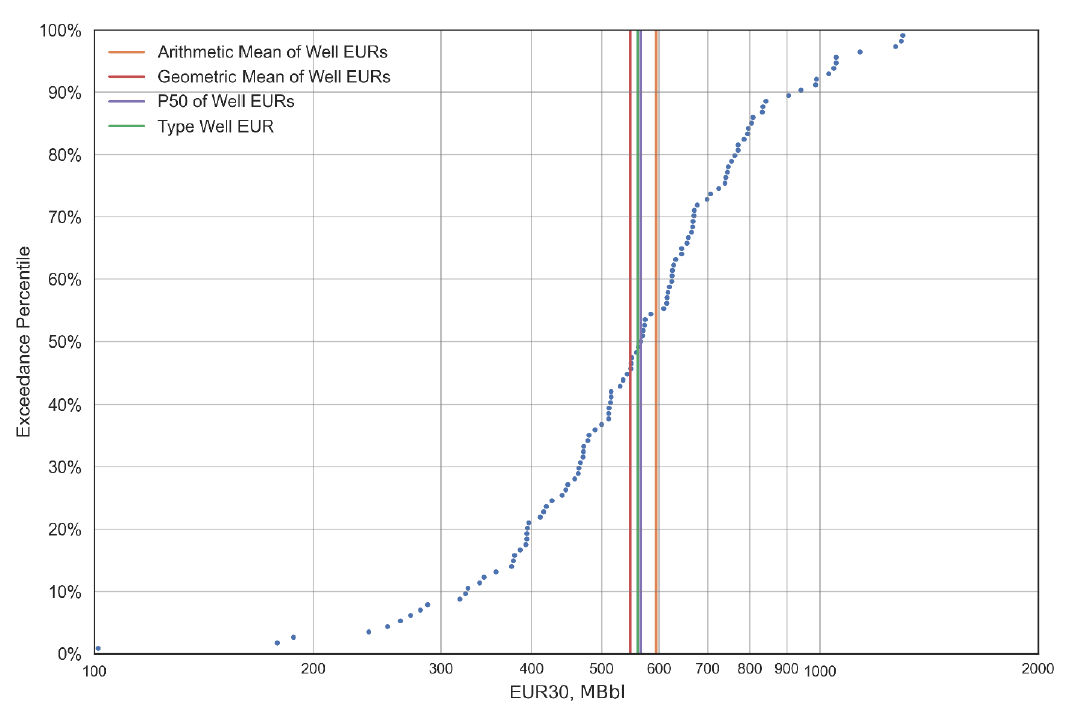
Step 6: Validate the TWP
Ensure the TWP accurately represents the typical well performance.
-
Process:
-
Compare the TWP time-rate profile to the P50, arithmetic mean, and geometric mean of the well set’s production profiles (See figure below).
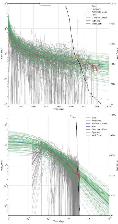
Figure 5. Time-rate profiles for all well data, all wells forecasts, central tendency measures, and the TWP.
-
Verify that the TWP EUR lies between the geometric mean and arithmetic mean of the well set’s EURs, ideally near the P50 (Figure 4).
-
Check for robustness against outliers by observing that the TWP is unaffected by extreme production rates (e.g., a single well’s rate spike at 2,750 days in Figure 5).
-
-
Considerations:
-
The TWP should avoid the overprediction bias seen in arithmetic mean-based methods, which are skewed by high-performing wells.
-
The paper demonstrates that the TWP closely matches the P50, indicating a statistically robust representation.
-
Step 7: Extend to Associated Phases (Optional)
Construct TWPs for associated phases (e.g., gas or water) if needed.
-
Process:
-
Use a power-law model (e.g., Fulford et al., 2022) to forecast ratios like gas-oil ratio (GOR), condensate-gas ratio (CGR), water-oil ratio (WOR), or water-gas ratio (WGR).
-
Apply transformations to the power-law model parameters:
-
Intercept or starting rate: Natural logarithm
-
Slope (equivalent to b-parameter): No transformation
-
-
Compute the arithmetic mean of the transformed parameters and reverse the transformations to obtain the TWP parameters for the associated phase.
-
-
Considerations:
-
Averaging associated phase rates directly (e.g., gas rates) introduces errors due to weighting by the primary phase (e.g., oil rate). The power-law model avoids this by modeling ratios.
-
GOR behavior is often more predictable than production rates, improving TWP accuracy for associated phases.
-
Key Features of the Parametric Method
-
Statistical Rigor: Uses linear regression with transformed parameters to eliminate biases from arithmetic averaging.
-
Robustness: The TWP is close to the P50, immune to outlier bias, and validated with a high R2 .
-
Flexibility: Applicable to primary and associated phases, with potential use for other decline models (e.g., hyperbolic) with calibration.
-
Automation: Eliminates subjective interpretation, enabling rapid, consistent TWP generation.
Constraints of the Parametric Method
-
Requires forecasting every well, which may be time-intensive initially but can be mitigated by pre-forecasting.
-
Industry software may not support full-life forecasting starting from initial production, requiring custom workflows.
-
The method assumes the THM is appropriate; other models may need additional calibration.
References:
-
Fulford, David S. "Construction of parametric type well profiles using linear models." In Unconventional Resources Technology Conference, 17–19 June 2024, pp. 797-810. Unconventional Resources Technology Conference (URTeC), 2024.
-
Russell, Boyd, and Randy Freeborn. "A Practical Guide to Unconventional Petroleum Evaluation Part 2." In SPE Canada Unconventional Resources Conference, pp. SPE-167215. SPE, 2013.
-
Freeborn, Randy, and Boyd Russell. "Creating more-representative type wells." SPE Economics & Management 8, no. 02 (2016): 50-58.
-
Fulford, D. S., and T. A. Blasingame. "Evaluation of time-rate performance of shale wells using the transient hyperbolic relation." In SPE Canada Unconventional Resources Conference, pp. SPE-167242. SPE, 2013.
-
Fulford, David S., Hamid Behmanesh, Christopher R. Clarkson, and Thomas A. Blasingame. "On the relationship between gas-oil ratio and well performance for unconventional reservoirs." In Unconventional Resources Technology Conference, 20–22 June 2022, pp. 2825-2854. Unconventional Resources Technology Conference (URTeC), 2022.