
Introduction
Pressure sensor drift refers to how much the sensor’s OUTPUT changes over time even when the measured pressure is remaining constant.
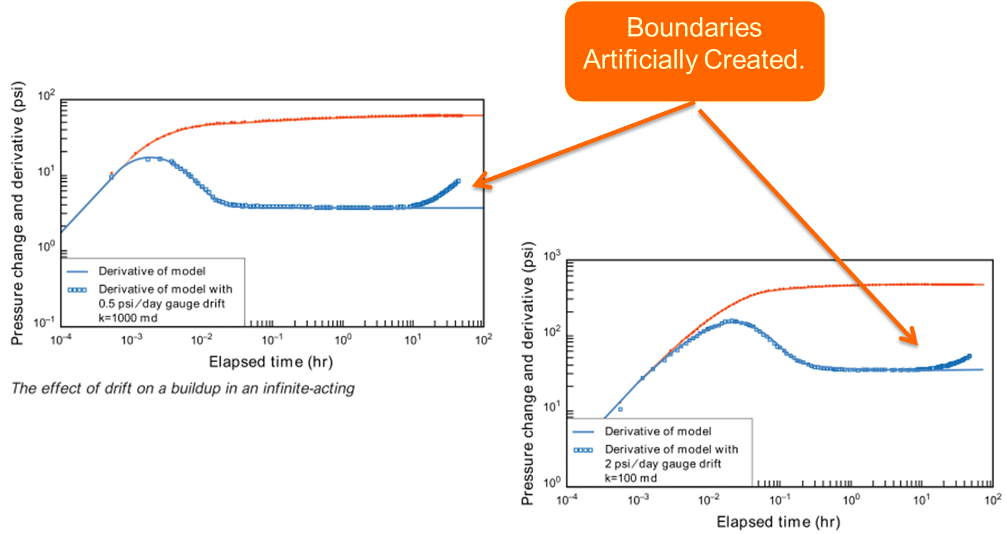
Example 1: False Boundaries
Using simulated data, a POSITIVE gauge drift was introduced in the measured BHP data for a constant rate well. As can be seen in the figures below, the Bourdet (Well Testing) Derivative inclines providing the illusion of increasing loss of Kh, or apparent boundaries.
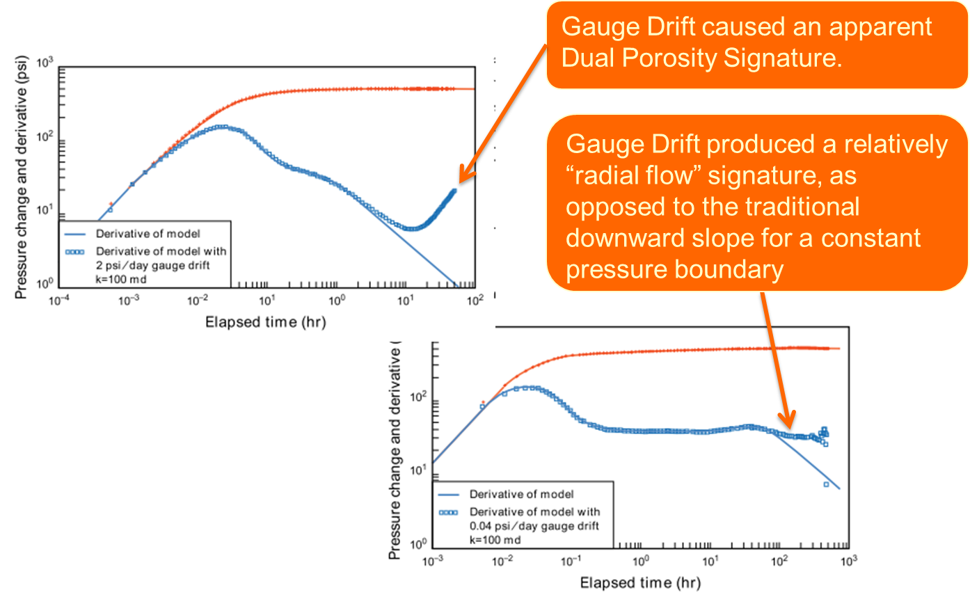
Example 2: False Heterogeneity
In the next two examples, a POSTIVE gauge drift was again added to the simulated data. In this scenario, a well was placed with a simple homogenous reservoir but with a constant pressure boundary (refer to Radial Flow Models for additional information).
-
In the first scenario, gauge drift produced a false Dual Porosity signature.
-
In the second scenario, gauge drift produced a false Radial Flow Models signature.
-
In both scenarios, the distance and type of reservoir boundary was obscured.
References:
Kruger, C., Heiam, B., Douglas, A., & Johnston, S. (2011). Data Quality & Acquisition Efficiency (Chapter 4)