Horizontal Well Models

Introduction

Horizontal wells (outside of the former Soviet Union) started in the 1980’s, and eventually become common place in early 1990’s

The main advantages of horizontal wells were:

• Increased productivity, compared to a vertical well, due to the length of the well

• Potentially reduce water and gas coning

• Intersect natural fractures

• Improve commercial success of low permeability reservoirs

• and more

Joshi/Economides et al Model

According to Joshi [1991] and Economides et al [1994], the following relationships were derived. Originally, Joshi presented his mathematical model considering steady-state flow in the horizontal plan, and pseudo-steady-state in the vertical plane.

For pseudo steady state:

Where Iani reflects the measurement of vertical-to-horizontal permeability. See CSG Permeability / Permeability Anisotropy for additional information of anisotropic examples.

and “a“ is a function the horizontal well drainage area (ellipsoid)

Helmy et al Model

Helmy and Wattenbarger [1998] presented a sophisticated model to calculate the productivity index of a horizontal well within an anisotropic reservoir allowing for”:

• Square and/or rectangular reservoir, allowing for greater flexibility in shape (i.e. channel shaped with the well in a corner or other combination). It can also be used to add vertical wells to the system as discussed here Extension to a Generalized Well Model

• Variable location in the x, y, and z-direction.

• Refer to the diagrams below for additional information

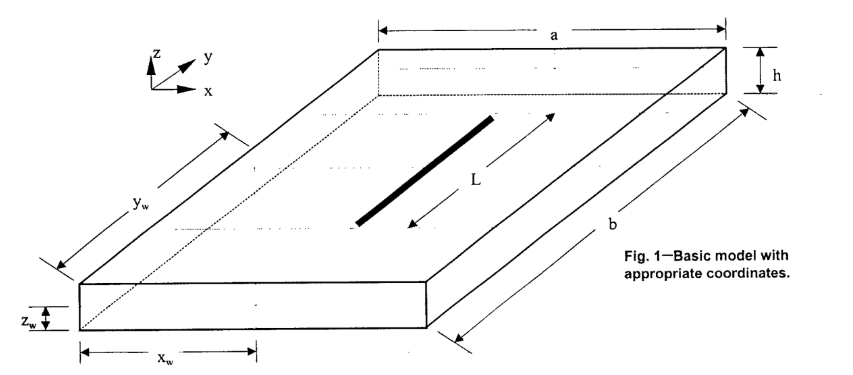
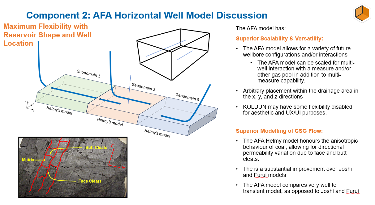
The Helmy model also provides superior performance with respect to Joshi/Economides and Furui models as shown below. A transient (well test) model was used for the Benchmark [Thompson et al, 1991]

Helmy vs Joshi/Economides vs Furui

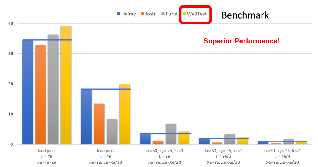
Basic Equations

Where:

= Numerically derived Shape factor

= partial penetration skin

The constant uses the standards conditions and algo carry some units conversions to express the gas flow rate in :

Helmy et al us an analytical solution to expand the Dietz Shape factor to a correlation approach for any combination of reservoir size, horizontal well size/location in xyz, and constant flowing pressure or constant rate boundary conditions. A correlation for was developed using numerical simulation.

For anisotropic conditions, transformed coordinates are used.

For x, y, and z coordinates

For coordinates of the horizontal well location

For coordinates / size of the rerserovir

Additional Comments:

Some authors such as Guo et al (2007) indicted that these types of models can be optimistic for higher productivity reservoirs if the effects of wellbore are neglected.

See Also:

References:

• Michael Economides, Xiuli Wang, Advanced Natural Gas Engineering, Gulf Publishing Company, 2009

• M. Wael Helmey, & R. A. Wattenbarger, Simplified Productivity Equations for Horizontal Wells Producing at Constant Rate and Constant Pressure.

• Joshi, S.D., 1991. Horizontal Well Technology. PennWell Publishing Company, Tulsa, OK.

• T. A. Blasingame, Analysis Well Performance, v20230723, Texas A&M

• "Efficient Algorithms for Computing the Bounded Reservoir Horizontal Well Pressure Responses", L.G. Thompson, J.L. Manrique and T.A. Jelmert, Paper SPE 21827 presented at 1991 Rocky Mountain Regional Meeting and Low-Permeability Reservoirs Symposium, Denver, CO, April 15 - 17.